Case Study 3 Trucking Industry What was the impact of deregulation - - PowerPoint PPT Presentation

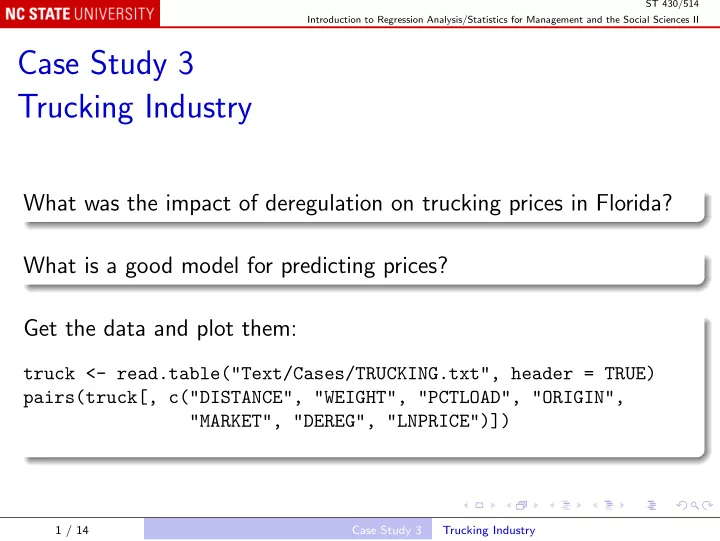
ST 430/514 Introduction to Regression Analysis/Statistics for Management and the Social Sciences II

Case Study 3 Trucking Industry

What was the impact of deregulation on trucking prices in Florida? What is a good model for predicting prices? Get the data and plot them:

truck <- read.table("Text/Cases/TRUCKING.txt", header = TRUE) pairs(truck[, c("DISTANCE", "WEIGHT", "PCTLOAD", "ORIGIN", "MARKET", "DEREG", "LNPRICE")])

1 / 14 Case Study 3 Trucking Industry

ST 430/514 Introduction to Regression Analysis/Statistics for Management and the Social Sciences II

The dependent variable will be LNPRICE = log(price per ton-mile) The study chooses to omit one variable, PRODUCT.

2 / 14 Case Study 3 Trucking Industry

ST 430/514 Introduction to Regression Analysis/Statistics for Management and the Social Sciences II

Use stepwise regression to screen the other variables:

truck$y <- truck$LNPRICE truck$x1 <- truck$DISTANCE truck$x2 <- truck$WEIGHT truck$x3 <- truck$DEREG truck$x4 <- truck$ORIGIN truck$x5 <- truck$PCTLOAD truck$x6 <- truck$MARKET start <- lm(y ~ 1, truck) firstOrder <- y ~ x1 + x2 + x3 + x4 + x5 + x6 summary(step(start, scope = firstOrder))

3 / 14 Case Study 3 Trucking Industry

ST 430/514 Introduction to Regression Analysis/Statistics for Management and the Social Sciences II

This identifies: x1, DISTANCE; x2, WEIGHT; x3, the DEREG indicator; x4, the ORIGIN indicator. Stepping down from the full first-order model, instead of stepping up from the empty model, finds the same variables:

summary(step(lm(firstOrder, truck), firstOrder))

4 / 14 Case Study 3 Trucking Industry

ST 430/514 Introduction to Regression Analysis/Statistics for Management and the Social Sciences II

The study continues with the full second order model in these variables:

lm1 <- lm(y ~ (x1 + x2 + x1:x2 + I(x1^2) + I(x2^2)) * x3 * x4, truck) summary(lm1)

Note that none of the 8 squared terms are significant; try dropping them:

lm2 <- lm(y ~ (x1 + x2 + x1:x2) * x3 * x4, truck) summary(lm2) anova(lm2, lm1)

R2 drops substantially, and F is highly significant, so the simpler model is rejected.

5 / 14 Case Study 3 Trucking Industry

ST 430/514 Introduction to Regression Analysis/Statistics for Management and the Social Sciences II

Next try dropping, from the full second order model, the interactions between quantitative and qualitative variables:

lm3 <- lm(y ~ x1 + x2 + x1:x2 + I(x1^2) + I(x2^2) + x3 * x4, truck) summary(lm3) anova(lm3, lm1)

Again F is significant, and the simpler model is rejected.

6 / 14 Case Study 3 Trucking Industry

ST 430/514 Introduction to Regression Analysis/Statistics for Management and the Social Sciences II

Next try: drop the interactions of the qualitative variables with only the squared terms:

lm4 <- lm(y ~ (x1 + x2 + x1:x2) * x3 * x4 + I(x1^2) + I(x2^2), truck) summary(lm4) anova(lm4, lm1)

Success! R2 drops only a little, and R2

a actually increases; also F is

not significant. This simpler model is not rejected.

7 / 14 Case Study 3 Trucking Industry

ST 430/514 Introduction to Regression Analysis/Statistics for Management and the Social Sciences II

Next, explore whether x4, ORIGIN, can be dropped from this simpler model:

lm5 <- lm(y ~ (x1 + x2 + x1:x2) * x3 + I(x1^2) + I(x2^2), truck) summary(lm5) anova(lm5, lm4)

F is highly significant, so we reject the simpler model.

8 / 14 Case Study 3 Trucking Industry

ST 430/514 Introduction to Regression Analysis/Statistics for Management and the Social Sciences II

Next, explore whether x3, DEREG, can be dropped:

lm6 <- lm(y ~ (x1 + x2 + x1:x2) * x4 + I(x1^2) + I(x2^2), truck) summary(lm6) anova(lm6, lm4)

Again, F is highly significant, so we reject the simpler model.

9 / 14 Case Study 3 Trucking Industry

ST 430/514 Introduction to Regression Analysis/Statistics for Management and the Social Sciences II

Finally, explore whether x3, DEREG, interacts with x4, ORIGIN, by dropping their interaction terms:

lm7 <- lm(y ~ (x1 + x2 + x1:x2) * (x3 + x4) + I(x1^2) + I(x2^2), truck) summary(lm7) anova(lm7, lm4)

This time, F is not significant, so the simpler model, without the interactions, is not rejected.

10 / 14 Case Study 3 Trucking Industry

ST 430/514 Introduction to Regression Analysis/Statistics for Management and the Social Sciences II

Model-building with step() Suppose we begin with the full second order model and simplify it using step() and BIC (same result using AIC):

stepLm1 <- step(lm1, direction = "both", k = log(nrow(truck))) summary(stepLm1)

The model looks complicated, but the formula is equivalent to y ~ (x1 + x2 + x1:x2) * x3 * x4 + I(x1^2):

summary(lm(y ~ (x1 + x2 + x1:x2) * x3 * x4 + I(x1^2), truck))

This is Model 4 with I(x2^2) dropped.

11 / 14 Case Study 3 Trucking Industry

ST 430/514 Introduction to Regression Analysis/Statistics for Management and the Social Sciences II

Without screening: Suppose we skip the screening stage, and just use step() with all six variables; using BIC:

secondOrder <- y ~ ((x1 + x2 + x5)^2 + I(x1^2) + I(x2^2) + I(x5^2)) * x3 * x4 * x6 stepBIC <- step(start, secondOrder, k = log(nrow(truck))) summary(stepBIC)

This model is the same as y ~ x1 + I(x1^2) + x2 * x3: quadratic function of x1 = DISTANCE + interaction of x2 = WEIGHT with x3 = DEREG

12 / 14 Case Study 3 Trucking Industry

ST 430/514 Introduction to Regression Analysis/Statistics for Management and the Social Sciences II

Using AIC:

stepAIC <- step(start, secondOrder) summary(stepAIC)

This more complicated model can be written y ~ (x1 + I(x1^2)) * x6 + x2 * x3. It is similar to the model found with BIC, but now the quadratic function of DISTANCE has different coefficients for each level of x6 = MARKET.

13 / 14 Case Study 3 Trucking Industry

ST 430/514 Introduction to Regression Analysis/Statistics for Management and the Social Sciences II

These models have slightly lower R2 than Models 4 or 7, but slightly better PRESS statistics. They show the effect of deregulation (x3) more clearly: intercept reduction of −0.69 (e−0.69 = 0.5); coefficient of WEIGHT (x2): -0.028 to -0.057.

14 / 14 Case Study 3 Trucking Industry