BS2247 Introduction to Econometrics Lecture 7: The multiple - PowerPoint PPT Presentation

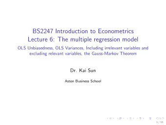
BS2247 Introduction to Econometrics Lecture 7: The multiple regression model Testing single linear hypothesis (i.e., t statistic, p -value, confidence intervals, etc.) Dr. Kai Sun Aston Business School 1 / 28

Why testing for hypothesis? ◮ OLS estimates, ˆ β ’s, are random variables - they are estimated from data, which are random draws from population. ◮ Intuitively, because ˆ β ’s are random, we want to test if they are close enough to a particular value. ◮ For example, if we obtained OLS estimate ˆ β 1 = 1 (i.e., the estimated β 1 is 1), we must keep in mind that the true β 1 may not necessarily be 1, although the true β 1 should be close to 1, such as 1.2, etc. ◮ Because we never know the true β 1 , we want to test if β 1 = 1 (or some other values) or not. 2 / 28

Why testing for hypothesis? ◮ OLS estimates, ˆ β ’s, are random variables - they are estimated from data, which are random draws from population. ◮ Intuitively, because ˆ β ’s are random, we want to test if they are close enough to a particular value. ◮ For example, if we obtained OLS estimate ˆ β 1 = 1 (i.e., the estimated β 1 is 1), we must keep in mind that the true β 1 may not necessarily be 1, although the true β 1 should be close to 1, such as 1.2, etc. ◮ Because we never know the true β 1 , we want to test if β 1 = 1 (or some other values) or not. 2 / 28

Why testing for hypothesis? ◮ OLS estimates, ˆ β ’s, are random variables - they are estimated from data, which are random draws from population. ◮ Intuitively, because ˆ β ’s are random, we want to test if they are close enough to a particular value. ◮ For example, if we obtained OLS estimate ˆ β 1 = 1 (i.e., the estimated β 1 is 1), we must keep in mind that the true β 1 may not necessarily be 1, although the true β 1 should be close to 1, such as 1.2, etc. ◮ Because we never know the true β 1 , we want to test if β 1 = 1 (or some other values) or not. 2 / 28

Why testing for hypothesis? ◮ OLS estimates, ˆ β ’s, are random variables - they are estimated from data, which are random draws from population. ◮ Intuitively, because ˆ β ’s are random, we want to test if they are close enough to a particular value. ◮ For example, if we obtained OLS estimate ˆ β 1 = 1 (i.e., the estimated β 1 is 1), we must keep in mind that the true β 1 may not necessarily be 1, although the true β 1 should be close to 1, such as 1.2, etc. ◮ Because we never know the true β 1 , we want to test if β 1 = 1 (or some other values) or not. 2 / 28

Assumptions of the Classical Linear Model (CLM) ◮ So far, we know that OLS estimator is unbiased under MLR.1-MLR.4 OLS estimator is BLUE under MLR.1-MLR.5 (i.e., the Gauss-Markov assumptions) ◮ In order to do classical hypothesis testing, we need to add another assumption: Assumption MLR.6: u is independent of x 1 , x 2 , . . . , x k , and u is normally distributed with zero mean and variance σ 2 : u ∼ N (0 , σ 2 ) 3 / 28

Assumptions of the Classical Linear Model (CLM) ◮ So far, we know that OLS estimator is unbiased under MLR.1-MLR.4 OLS estimator is BLUE under MLR.1-MLR.5 (i.e., the Gauss-Markov assumptions) ◮ In order to do classical hypothesis testing, we need to add another assumption: Assumption MLR.6: u is independent of x 1 , x 2 , . . . , x k , and u is normally distributed with zero mean and variance σ 2 : u ∼ N (0 , σ 2 ) 3 / 28

◮ MLR.6 also means that u | x 1 , . . . , x k ∼ N (0 , σ 2 ), or y | x 1 , . . . , x k ∼ N ( β 0 + β 1 x 1 + . . . + β k x k , σ 2 ) ◮ Assumption MLR.1-MLR.6: Classical Linear Model (CLM) assumptions ◮ Under the CLM assumptions, OLS estimator is not only BLUE, but is the minimum variance unbiased estimator (MVUE) - the model may not necessarily be linear in parameter! ◮ For large sample, the normality assumption of u becomes less important. But here we just make the normality assumption. 4 / 28

◮ MLR.6 also means that u | x 1 , . . . , x k ∼ N (0 , σ 2 ), or y | x 1 , . . . , x k ∼ N ( β 0 + β 1 x 1 + . . . + β k x k , σ 2 ) ◮ Assumption MLR.1-MLR.6: Classical Linear Model (CLM) assumptions ◮ Under the CLM assumptions, OLS estimator is not only BLUE, but is the minimum variance unbiased estimator (MVUE) - the model may not necessarily be linear in parameter! ◮ For large sample, the normality assumption of u becomes less important. But here we just make the normality assumption. 4 / 28

◮ MLR.6 also means that u | x 1 , . . . , x k ∼ N (0 , σ 2 ), or y | x 1 , . . . , x k ∼ N ( β 0 + β 1 x 1 + . . . + β k x k , σ 2 ) ◮ Assumption MLR.1-MLR.6: Classical Linear Model (CLM) assumptions ◮ Under the CLM assumptions, OLS estimator is not only BLUE, but is the minimum variance unbiased estimator (MVUE) - the model may not necessarily be linear in parameter! ◮ For large sample, the normality assumption of u becomes less important. But here we just make the normality assumption. 4 / 28

◮ MLR.6 also means that u | x 1 , . . . , x k ∼ N (0 , σ 2 ), or y | x 1 , . . . , x k ∼ N ( β 0 + β 1 x 1 + . . . + β k x k , σ 2 ) ◮ Assumption MLR.1-MLR.6: Classical Linear Model (CLM) assumptions ◮ Under the CLM assumptions, OLS estimator is not only BLUE, but is the minimum variance unbiased estimator (MVUE) - the model may not necessarily be linear in parameter! ◮ For large sample, the normality assumption of u becomes less important. But here we just make the normality assumption. 4 / 28

Distribution of ˆ β ◮ Under the CLM assumptions, it can be shown that β | x ∼ N ( β, Var (ˆ ˆ β | x )) ◮ In the simple regression case, we have β 1 = � x ) 2 y i = � ˆ x i − ¯ x � i a i y i i i ( x i − ¯ ˆ β 1 is a linear combination of y i “If a random variable is a linear combination of a normally distributed random variable, then this random variable is also normally distributed.” 5 / 28

Distribution of ˆ β ◮ Under the CLM assumptions, it can be shown that β | x ∼ N ( β, Var (ˆ ˆ β | x )) ◮ In the simple regression case, we have β 1 = � x ) 2 y i = � ˆ x i − ¯ x � i a i y i i i ( x i − ¯ ˆ β 1 is a linear combination of y i “If a random variable is a linear combination of a normally distributed random variable, then this random variable is also normally distributed.” 5 / 28

Distribution of ˆ β ◮ Under the CLM assumptions, it can be shown that β | x ∼ N ( β, Var (ˆ ˆ β | x )) ◮ In the simple regression case, we have β 1 = � x ) 2 y i = � ˆ x i − ¯ x � i a i y i i i ( x i − ¯ ˆ β 1 is a linear combination of y i “If a random variable is a linear combination of a normally distributed random variable, then this random variable is also normally distributed.” 5 / 28

◮ Similarly, in the multiple regression case, we have β j | x 1 , . . . , x k ∼ N ( β j , Var (ˆ ˆ β j | x 1 , . . . , x k )) ◮ Standardize ˆ β j , ˆ β j − β j ∼ N (0 , 1) sd (ˆ β j ) 6 / 28

The t Test � ◮ Replace sd (ˆ Var (ˆ β j ) (which depends on true σ 2 ) with β j ) = � se (ˆ Var (ˆ � β j ) (which depends on the estimated σ 2 , ˆ σ 2 ), β j ) = we can get a calculated t statistic: ˆ β j − β j t CALC = β j ) ∼ t n − k − 1 se (ˆ ◮ We used se ( · ) instead of sd ( · ) is because σ 2 is unknown, and we have to estimate it. ◮ Degrees of freedom (DF) = n-(k+1) = the number of observations - the number of parameters (i.e., number of “free” observations) 7 / 28

The t Test � ◮ Replace sd (ˆ Var (ˆ β j ) (which depends on true σ 2 ) with β j ) = � se (ˆ Var (ˆ � β j ) (which depends on the estimated σ 2 , ˆ σ 2 ), β j ) = we can get a calculated t statistic: ˆ β j − β j t CALC = β j ) ∼ t n − k − 1 se (ˆ ◮ We used se ( · ) instead of sd ( · ) is because σ 2 is unknown, and we have to estimate it. ◮ Degrees of freedom (DF) = n-(k+1) = the number of observations - the number of parameters (i.e., number of “free” observations) 7 / 28

The t Test � ◮ Replace sd (ˆ Var (ˆ β j ) (which depends on true σ 2 ) with β j ) = � se (ˆ Var (ˆ � β j ) (which depends on the estimated σ 2 , ˆ σ 2 ), β j ) = we can get a calculated t statistic: ˆ β j − β j t CALC = β j ) ∼ t n − k − 1 se (ˆ ◮ We used se ( · ) instead of sd ( · ) is because σ 2 is unknown, and we have to estimate it. ◮ Degrees of freedom (DF) = n-(k+1) = the number of observations - the number of parameters (i.e., number of “free” observations) 7 / 28

◮ Knowing the sampling distribution for the standardized estimator allows us to carry out hypothesis tests ◮ First, state a null hypothesis, for example, H 0 : β j = 0 (CANNOT write as ˆ β j = 0) If accept null, then accept that x j has no effect on y , controlling for other x ’s ◮ Second, form the calculated t statistic: ˆ β j − 0 t CALC = se (ˆ β j ) 8 / 28

◮ Knowing the sampling distribution for the standardized estimator allows us to carry out hypothesis tests ◮ First, state a null hypothesis, for example, H 0 : β j = 0 (CANNOT write as ˆ β j = 0) If accept null, then accept that x j has no effect on y , controlling for other x ’s ◮ Second, form the calculated t statistic: ˆ β j − 0 t CALC = se (ˆ β j ) 8 / 28