Branch and Bound CS31005: Algorithms-II Autumn 2020 IIT Kharagpur - PowerPoint PPT Presentation
Branch and Bound CS31005: Algorithms-II Autumn 2020 IIT Kharagpur Branch and Bound An algorithm design technique, primarily for solving hard optimization problems Guarantees that the optimal solution will be found Does not
Branch and Bound CS31005: Algorithms-II Autumn 2020 IIT Kharagpur
Branch and Bound An algorithm design technique, primarily for solving hard optimization problems Guarantees that the optimal solution will be found Does not necessarily guarantee worst case polynomial time complexity But tries to ensure faster time on most instances Basic Idea Model the entire solution space as a tree Search for a solution in the tree systematically, eliminating parts of the tree from the search intelligently Important technique for solving many problems for which efficient algorithms (worst case polynomial time) are not known
Optimization Problems Set of input variables I Set of output variables O Values of the output variables define the solution space Set of constraints C over the variables Set of feasible solutions S Set of solutions that satisfy all the constraints Objective function F : S → R (also called cost function ) Gives a value F(s) for each solution s ∈ S Optimal solution A solution s ∈ S for which F ( s ) is maximum among all s ∈ S (for a maximization problem) or minimum (for a minimization problem)
Example Many problems that you have seen so far Minimum weight spanning tree, matrix chain multiplication, longest common subsequence, fractional knapsack problem, …. All these (that you have seen in Algorithms-1 course) have known efficient algorithms Graph Coloring Input: an undirected graph Output: a color assigned to each vertex Constraint: no two adjacent vertices have the same color Objective function: no of colors used by a feasible solution Goal: Find a coloring that uses the minimum number of colors No efficient algorithm known for general graphs
Bin Packing Input: a set of items X = { x 1 , x 2 , …. x n } with volume { v 1 , v 2 , v n } respectively, and set of bins B , each of volume V Output: an assignment of the items to bins (each item can be placed in exactly one bin) Constraint: the total volume of items placed in any bin must be ≤ V Objective function: number of bins used Goal: find an assignment of items to bins that uses the minimum number of bins No efficient algorithm known Note that a maximization problem can be transformed into a minimization function (and vice-versa) by just changing the sign of the objective function
Solution Structure For many optimization problems, the solution can be expressed as a n -tuple < x 1 , x 2 , …. x n > where each x i is chosen from some finite set S i Let size of S i be m i Then size of the solution space = m 1 m 2 m 3 …. m n Some of these solutions are feasible, some are infeasible Brute force approach Search the entire space for feasible solutions Compute the cost function for each feasible solution found Choose the one that maximizes/minimizes the objective function Problem: Solution space size may be too large
Example: 0-1 Knapsack Problem Given a set of n items 1, 2, … n with weights w 1 , w 2 , …, w n and values v 1 , v 2 , v n respectively , and a knapsack with total weight capacity W , find the largest subset of items that can be packed into the knapsack such that the total value gained is maximized. Solution format < x 1 , x 2 ,…., x n > x i = 1 if item i is chosen in the subset, 0 otherwise Feasible solution: ∑ x i w i ≤ W Objective function F : ∑ x i v i Optimal solution: feasible solution with maximum value of ∑ x i v i Solution space size 2 n
Example: Travelling Salesman Problem Given a complete weighted graph G = (V , E), find a Hamiltonian Cycle with the lowest total weight Suppose that the vertices are numbered 1, 2, …,|V|= n Solution format < x 1 , x 2 ,…., x n > x i ∈ {1, 2, …, n } gives the i -th vertex visited in the cycle Feasible solution: x i ≠ x j for any i ≠ j Objective function F : ∑ 1 ≤ i < n w ( x i , x i +1 ) + w ( x n , x 1 ), where w ( i , j ) is the weight of edge ( i , j ) Optimal solution: feasible solution with minimum value of objective function Solution space size ( n -1)!
State Space Tree Represent the solution space as a tree Each edge represents a choice of one x i Level 0 to Level 1 edges show choice of x 1 Level 1 to Level 2 edges show choice of x 2 Level i − 1 to Level i edges show choice of x i Each internal node represents a partial solution Partitions the solution space into disjoint subspaces Leaf nodes represent the complete solution (may or may not be feasible) Models the complete solution being built by choosing one component at a time
Example: 0-1 Knapsack Level 0 to Level 1 edges show choice of w 1 Level 1 to Level 2 edges show choice of w 2 Level i − 1 to Level i edges show choice of w i Level 0 (root) node partitions the solution space into those that contain w 1 and those that do not contain w 1 For the subtree which has w 1 chosen, Level 1 nodes partitions the subspace ( w 1 present) further into ( w 1 and w 2 present) and ( w 1 present but w 2 not present) Leaf nodes represent the solutions (the path from root to leaf shows what items are chosen (edges marked 1 along the path)
Finding the Optimal Solution One possible approach Generate the state space tree, look at all solutions (leaf nodes), find the feasible solutions, apply objective function on each feasible solution, and choose the optimal But generating the tree is as good as doing brute force search Will take huge space (to store the tree) and huge time (to generate all nodes) Need to do something better To reduce space, do not generate all nodes at once To reduce time, do not generate all nodes (how to decide?) We will first look at the problem of finding just one feasible solution to understand a basic technique
Finding One Feasible Solution
Basic Approach Expand the tree systematically in parts, stop when you find a feasible solution Reduces space as whole tree is not generated at one go The parts that have been looked at already are not stored May reduce time for many instances as feasible solution may be found without generating the whole tree But in worst case, you may still have to generate all the nodes
How to expand the tree? Start with root node Generate other nodes in some order DFS, BFS, …. Live node: a node which is generated but all children of which has not been generated Dead node: A generated node which is not to be expanded (will see why later) or whose all children have been generated The different node generation orders will pick one live node to expand (generate its children) at one time E-node: The live node being expanded currently
Example: n -Queens Problem Consider a n × n board You have to place n queens on the n × n squares so that no two queens can attack each other, i.e., no two queens should be In the same row In the same column In the same diagonal
One Solution for 8-queens Courtesy: Computer Algorithms: E. Horowitz, S. Sahni, and S. Rajasekharan
How to find a solution? Say queens are numbered 1 to n Rows and columns are also numbered from 1 to n Without loss of generality, assume that queen i is placed in row i So need to find the column in which each queen i needs to be placed Solution format: ( x 1 , x 2 , …. x n ) where x i gives the column no. that queen i is placed in So x i ∈ {1, 2, 3, …., n }
State Space Tree for 4-Queens Generated in DFS order (no. inside node shows order) Courtesy: Computer Algorithms: E. Horowitz, S. Sahni, and S. Rajasekharan
But do we need to explore the entire tree? Consider the node marked 3, corresponding to the choices (made so far) of x 1 = 1, x 2 = 2 But this cannot lead to any feasible solution Queen 1 and 2 are on same diagonal Cannot be feasible irrespective of the consequent choice of x 3 , x 4 ,…. So while generating the tree, no need to generate the subtree rooted at node 3 Many other such cases in the tree… Can prune (not generate) large parts of the tree, saving time
Pruned Tree Courtesy: Computer Algorithms: E. Horowitz, S. Sahni, and S. Rajasekharan
Backtracking Systematic search of the state space tree with pruning Pruning done using bounding functions Tree generated using DFS order When a child C of the current E-node R is generated, C becomes the new E-node R will become the E-node again after subtree rooted at C is fully explored At every step, apply the bounding function (a predicate) on a node to check if the subtree rooted at the node needs to be explored Do not generate the subtree rooted at the node if the bounding function returns false Find all feasible solutions (or stop at the first one if only one is needed)
Recommend
More recommend
Explore More Topics
Stay informed with curated content and fresh updates.
