Brain Connectivity-Informed Adaptive Regularization for Generalized - PowerPoint PPT Presentation
Brain Connectivity-Informed Adaptive Regularization for Generalized Outcomes Jaroslaw Harezlak, Ph.D. Professor and Interim Co-Chair Department of Epidemiology and Biostatistics Indiana University School of Public Health Bloomington, IN, USA
Brain Connectivity-Informed Adaptive Regularization for Generalized Outcomes Jaroslaw Harezlak, Ph.D. Professor and Interim Co-Chair Department of Epidemiology and Biostatistics Indiana University School of Public Health Bloomington, IN, USA May 22, 2020 Jaroslaw Harezlak May 22, 2020 1 / 33
Outline 1 Motivating application 2 Brain structure and connectivity 3 Regularization methods 4 riPEER - ridgified Partially Empirical Eigenvectors for Regression 5 Simulation study 6 Brain structure and HIV infection 7 Discussion Jaroslaw Harezlak May 22, 2020 2 / 33
HIV infection study - WUSM 1 N = 299 HIV-infected individuals: 228 males, 71 females ◮ Duration of infection range: 0 - 33y (mean: 10.2, sd: 8.7) ◮ Age range: 18 - 84 y.o. (mean: 42.3, sd: 16) 2 Imaging modalities ◮ T1 - anatomy ◮ DTI - structural connectivity Jaroslaw Harezlak May 22, 2020 3 / 33
Anatomy and connectivity 1 Anatomy ◮ MPRAGE protocol ◮ Processing using FreeSurfer software (version 5.1) ◮ Desikan-Killiany atlas - 66 cortical regions 2 Structural connectivity ◮ DTI and maximal diffusion coherence model ◮ Density of connections between each pair of regions Jaroslaw Harezlak May 22, 2020 4 / 33
MRI data Jaroslaw Harezlak May 22, 2020 5 / 33
MRI-derived data: cortical thickness 1 Parcellation of the cortex into 66 regions 2 Average cortical thickness (a) Parcellation of the brain (b) Cortical thickness Jaroslaw Harezlak May 22, 2020 6 / 33
Connections in the brain Jaroslaw Harezlak May 22, 2020 7 / 33
Connectivity matrices (a) Connectivity matrix: subject 1 (b) Connectivity matrix: subject 2 Jaroslaw Harezlak May 22, 2020 8 / 33
Population connectivity matrix STRONG A = 𝑏 𝑗𝑘 WEAK Jaroslaw Harezlak May 22, 2020 9 / 33
Questions 1 Scientific ◮ Are changes in the brain structure associated with the HIV infection? ◮ Is there any additional information provided by the structural connectivity? 2 Statistical ◮ How to deal with the highly correlated predictors in the regression models? ◮ How to incorporate the structural connectivity information in the regression models? Jaroslaw Harezlak May 22, 2020 10 / 33
Statistical model 1 y – n -dimensional response (e.g. NP domain score) 2 Z ∈ R n × 66 and X ∈ R n × m � 0 , σ 2 I n � for some unknown σ 2 > 0 3 ε ∼ N Jaroslaw Harezlak May 22, 2020 11 / 33
Statistical model 1 y – n -dimensional response (e.g. NP domain score) 2 Z ∈ R n × 66 and X ∈ R n × m � 0 , σ 2 I n � for some unknown σ 2 > 0 3 ε ∼ N Jaroslaw Harezlak May 22, 2020 12 / 33
Penalized estimation To find the estimates of b and β , we consider the optimization problem of the form � � � � � 2 � y − Zb − X β arg min + λ g ( b ) . 2 ���� � �� � b ,β penalty on b model fit term 1 g ( b ) = � i b 2 − → Ridge estimate i 2 g ( b ) = � i | b i | − → LASSO estimate 3 g ( b ) = || Lb || 2 − → Generalized ridge 2 T. W. Randolph, J. Harezlak, Z. Feng, Structured penalties for functional linear models – partially empirical eigenvectors for regression, Electronic Journal of Statistics (2012) Jaroslaw Harezlak May 22, 2020 13 / 33
Desired property of the estimate, ˆ b “Stronger connections between the brain regions i and j result in more similar coefficients ˆ b i and ˆ b j .” Jaroslaw Harezlak May 22, 2020 14 / 33
Penalty selection The natural choice of the penalty is � � b i − b j � 2 . g ( b ) = a ij i , j 1 d i := � k A ik . 2 D := diag � d 1 , . . . , d 66 � 3 Q := D − A [Laplacian of A] Then: � � b i − b j � 2 = b T Qb . a ij i , j Jaroslaw Harezlak May 22, 2020 15 / 33
Connections with the linear mixed models (LMM) Our objective function becomes �� � � � 2 � y − Zb − X β 2 + λ b T Qb arg min . b ,β This optimization problem is “equivalent” to the LMM formulation 1 y = Zb + X β + ε , where β is a vector of fixed effects and b a vector of random effects, 2 ε ∼ N � 0 , σ 2 I � , 3 b ∼ N � b Q − 1 � 0 , σ 2 , 4 λ , σ and σ b λ = σ 2 /σ 2 are connected via b . Jaroslaw Harezlak May 22, 2020 16 / 33
Selection of the regularization parameter Jaroslaw Harezlak May 22, 2020 17 / 33
The method riPEER (ridgified Partially Empirical Eigenvectors for Regression) � � �� � � ˆ � 2 b rP � y − Zb − X β 2 + λ Q b T Qb + λ R � b � 2 := arg min ˆ 2 � �� � β rP � �� � b ,β ridge part graph part b : λ Q b T Qb + λ R � b � 2 Figure 3: Different shapes of the set � 2 ≤ 1 � for p = 2. Jaroslaw Harezlak May 22, 2020 18 / 33
Connections with the linear mixed models (LMM) riPEER (ridgified Partially Empirical Eigenvectors for Regression) � ˆ � �� � � 2 + b T � λ Q Q + λ R I � b b � 2 rP � y − Zb − X β := arg min ˆ β rP b ,β This problem is “equivalent” to the LMM formulation 1 y = Zb + X β + ε , where β is a vector of fixed effects and b a vector of random effects, 2 ε ∼ N � 0 , σ 2 I � , � R I � − 1 � 0 , � 3 b ∼ N σ 2 Q Q + σ 2 , 4 λ Q λ R , σ , σ Q and σ R are connected via λ Q = σ 2 /σ 2 Q , λ R = σ 2 /σ 2 R . Jaroslaw Harezlak May 22, 2020 19 / 33
Simulation scheme SIMULATED SIGNAL ESTIMATION Graph given by adjacency matrix A Distorted graph 0.1 1 5 1 5 0.1 0.4 0.4 0.3 0.3 2 2 0.1 4 0.1 4 0.6 3 0.6 3 Laplacian : 𝑅 𝑢𝑠𝑣𝑓 Laplacian of distorted graph was used to find the estimate, 𝑐 „Invertible Laplacian ” : MSEr defined as 𝑅 𝑢𝑠𝑣𝑓 ≔ 𝑅 𝑢𝑠𝑣𝑓 + 0.001 ∙ 𝐽 2 𝑐 − 𝑐 𝑢𝑠𝑣𝑓 MSEr: = E 2 2 𝑐 𝑢𝑠𝑣𝑓 2 True signal used in simulation: 2 −1 ) as a measure of estimation accuracy 𝑐 𝑢𝑠𝑣𝑓 ~𝑂(0, 𝜏 𝑐 𝑅 𝑢𝑠𝑣𝑓 Jaroslaw Harezlak May 22, 2020 20 / 33
Simulation scheme – distorted connectivity matrices Jaroslaw Harezlak May 22, 2020 21 / 33
Simulation scheme Three methods compared: 1 ridge: λ Q := 0 (connectivity information is not used) 2 naive: λ R := 0, Q → � Q (only λ Q is selected) 3 riPEER (both lambdas are selected in an adaptive way) Axis of the plot 1 X axis: number of removed/added connections diss ( A true , A obs ) := number of all nonzero connections in A true � � � ˆ b − b true � 2 2 Y axis: MSEr := E 2 . � b true � 2 2 Jaroslaw Harezlak May 22, 2020 22 / 33
Simulation results 0.3 ridge b estimation MSEr 0.2 0.1 0.0 0.00 0.25 0.50 0.75 dissimilarity between A true and A obs Jaroslaw Harezlak May 22, 2020 23 / 33
Simulation results 0.3 ridge naive b estimation MSEr 0.2 0.1 0.0 0.00 0.25 0.50 0.75 dissimilarity between A true and A obs Jaroslaw Harezlak May 22, 2020 24 / 33
Simulation results 0.3 ridge naive ● riPEER b estimation MSEr 0.2 ● ● ● ● 0.1 ● ● ● 0.0 0.00 0.25 0.50 0.75 dissimilarity between A true and A obs Jaroslaw Harezlak May 22, 2020 25 / 33
Results: HIV study 1 Association between cortical thickness and speed of information processing 2 66 considered brain’s regions 3 N = 199 individuals Jaroslaw Harezlak May 22, 2020 26 / 33
Results: Speed of Information Processing caudalanteriorcingulate[L] caudalmiddlefrontal[L] bankssts[L] -0.05 0.05 0 medialorbitofrontal[L], posteriorcingulate[R] superiorparietal[R], supramarginal[R], superiorparietal[L], lateralorbitofrontal[R], precentral[R], Cortical regions: lingual[L], precentral[L], Jaroslaw Harezlak cuneus[L] entorhinal[L] inferiorparietal[L] fusiform[L] inferiortemporal[L] isthmuscingulate[L] lateraloccipital[L] lateralorbitofrontal[L] medialorbitofrontal[L] middletemporal[L] lingual[L] parahippocampal[L] paracentral[L] parsopercularis[L] parsorbitalis[L] parstriangularis[L] pericalcarine[L] posteriorcingulate[L] postcentral[L] rostralanteriorcingulate[L] precentral[L] rostralmiddlefrontal[L] precuneus[L] superiorfrontal[L] superiorparietal[L] superiortemporal[L] supramarginal[L] frontalpole[L] transversetemporal[L] temporalpole[L] caudalanteriorcingulate[R] riPEER estimate of b caudalmiddlefrontal[R] bankssts[R] cuneus[R] entorhinal[R] inferiorparietal[R] fusiform[R] inferiortemporal[R] isthmuscingulate[R] lateraloccipital[R] lateralorbitofrontal[R] medialorbitofrontal[R] middletemporal[R] lingual[R] parahippocampal[R] paracentral[R] parsopercularis[R] parsorbitalis[R] parstriangularis[R] pericalcarine[R] posteriorcingulate[R] postcentral[R] May 22, 2020 rostralanteriorcingulate[R] precentral[R] rostralmiddlefrontal[R] precuneus[R] superiorfrontal[R] superiorparietal[R] superiortemporal[R] supramarginal[R] frontalpole[R] transversetemporal[R] temporalpole[R] 27 / 33
Non-Gaussian distributions y i ∼ member of an Exponential family of distribution Consider an optimization problem of the form � � − 2 loglik ( y ; β, b ) arg min + g λ ( b ) . � �� � � �� � b ,β model fit term penalty on b g λ ( b ) := λ Q b T Qb + λ R � b � 2 2 λ Q and λ R are selected based on the equivalence with GLMM Jaroslaw Harezlak May 22, 2020 28 / 33
Recommend
More recommend
Explore More Topics
Stay informed with curated content and fresh updates.
