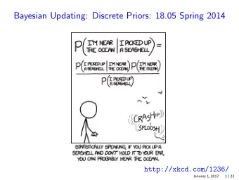
Bayesian Updating: Continuous Priors 18.05 Spring 2014 Jeremy Orloff - PowerPoint PPT Presentation
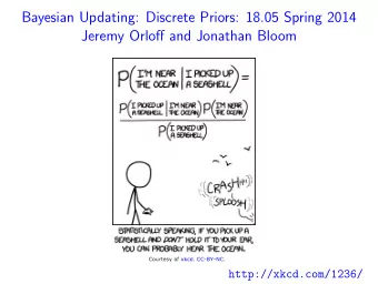
Bayesian Updating: Continuous Priors 18.05 Spring 2014 Jeremy Orloff and Jonathan Bloom Problem 6a on pset 5 Mrs S is found stabbed in her family garden. Mr S behaves strangely after her death and is considered as a suspect. Investigation shows that
Bayesian Updating: Continuous Priors 18.05 Spring 2014 Jeremy Orloff and Jonathan Bloom
Problem 6a on pset 5 Mrs S is found stabbed in her family garden. Mr S behaves strangely after her death and is considered as a suspect. Investigation shows that Mr S had beaten up his wife on at least nine previous occasions. The prosecution advances this data as evidence in favor of the hypothesis that Mr S is guilty of the murder. Mr S’s highly paid lawyer say, ‘ statistically , only one in a thousand wife-beaters actually goes on to murder his wife. So the wife-beating is not strong evidence at all. In fact, given the wife beating evidence alone, it’s extremely unlikely that he would be the murderer of his wife – only a 1/1000 chance. You should therefore find him innocent.’ What do you think of the lawyers argument? May 29, 2014 2 / 13
Problem 6b on pset 5 In 1999 in Great Britain, Sally Clark was convicted of murdering her two sons after each child died weeks after birth (the first in 1996, the second in 1998). Her conviction was largely based on the testimony of the pediatrician Professor Sir Roy Meadow. He claimed that, for an affluent non-smoking family like the Clarks, the probability of a single cot death (SIDS) was 1 in 8543, so the probability of two cot deaths in the same family was around “1 in 73 million.” Given that there are around 700,000 live births in Britain each year, Meadow argued that a double cot death would be expected to occur once every hundred years. Finally, he reasoned that given this vanishingly small rate, the far more likely scenario is that Sally Clark murdered her children. May 29, 2014 3 / 13
Continuous range of hypotheses Example. Bernoulli with unknown probability of success p . Can hypothesize that p takes any value in [0 , 1]. Model: ‘bent coin’ with probability p of heads. Example. Waiting time X ∼ exp( λ ) with unknown λ . Can hypothesize any λ > 0. Example. Have normal random variable with unknown µ and σ . Can hypothesisze ( µ, σ ) anywhere in ( −∞ , ∞ ) × [0 , ∞ ). May 29, 2014 4 / 13
Review of pdf and probability X random variable with pdf f ( x ). f ( x ) is a density , units: probability/units of x . f ( x ) f ( x ) probability f ( x ) dx P ( c ≤ X ≤ d ) dx x x c d x d P ( c ≤ X ≤ d ) = f ( x ) dx . c Probability X is in an infitesimal range dx around x is f ( x ) dx Often use probability f ( x ) dx instead of density f ( x ) May 29, 2014 5 / 13
Notational clarity for continuous parameters Example. Suppose that X ∼ Bernoulli( θ ), where θ is an unknown parameter. We can hypothesize that θ takes any value in [0 , 1]. We use θ instead of p because it’s neutral with no confusing connotations. Since θ is continuous we need a prior pdf f ( θ ). Use f ( θ ) d θ to work with probabilities instead of densities, e.g. θ is f ( . 5) d θ . The prior probability that θ is in the range . 5 ± d 2 To avoid cumbersome language we will say θ has prior probability f ( θ ) d θ .’ ‘The hypothesis θ ± d 2 May 29, 2014 6 / 13
Concept question Suppose X ∼ Bernoulli( θ ) where the value of θ is unknown. If we use Bayesian methods to make probabilistic statements about θ then which of the following is true? 1. The random variable is discrete, the space of hypotheses is discrete. 2. The random variable is discrete, the space of hypotheses is continuous. 3. The random variable is continuous, the space of hypotheses is discrete. 4. The random variable is continuous, the space of hypotheses is continuous. May 29, 2014 7 / 13
Bayesian update tables: discrete priors Discrete hypotheses: A , B , C . Data: D . Prior probability function: P ( A ), P ( B ), P ( C ). unnormalized hypothesis prior likelihood posterior posterior P ( D | A ) P ( A ) A P ( A ) P ( D| A ) P ( D| A ) P ( A ) P ( D ) P ( D | B ) P ( B ) B P ( B ) P ( D| B ) P ( D| B ) P ( B ) P ( D ) P ( D | C ) P ( C ) C P ( C ) P ( D| C ) P ( D| C ) P ( C ) P ( D ) Total 1 P ( D ) = sum 1 Note T = P ( D ) = the prior predictive probability of D . May 29, 2014 8 / 13
Bayesian update tables: continuous priors X ∼ Bernoulli( θ ). Unknown θ Continuous hypotheses θ in [0,1]. Data x . Prior pdf f ( θ ). Likelihood p ( x | θ ). hypoth. prior un. posterior posterior likel. p ( x | θ ) f ( θ ) dθ θ ± dθ f ( θ ) dθ p ( x | θ ) p ( x | θ ) f ( θ ) dθ 2 T 1 Total 1 T = p ( x | θ ) f ( θ ) dθ 1 0 ; Note T = p ( x ), the prior predictive probability of x . May 29, 2014 9 / 13
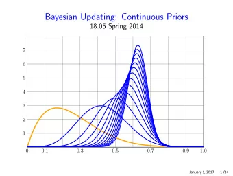
Example ‘Bent’ coin: unknown probability θ of heads. Flat prior: f ( θ ) = 1 on [0 , 1]. Data: toss once and get heads. unnormalized hypoth. prior likelihood posterior posterior θ ± d θ d θ θ θ d θ 2 θ d θ 2 f 1 Total 1 0 θ d θ = 1 / 2 1 Posterior pdf = f ( θ | x ) = 2 θ . (Should graph this.) May 29, 2014 10 / 13
Board question ‘Bent’ coin: unknown probability θ of heads. Prior: f ( θ ) = 2 θ on [0 , 1]. (This is the posterior from the last example.) Data: toss (again) and get heads. 1. Find the posterior pdf to this new data. 2. Suppose you toss again and get tails. Update your posterior from problem 1 using this data. 3. On one set of axes graph the prior and the posteriors from problems 1 and 2. May 29, 2014 11 / 13
Board Question Same scenario: bent coin ∼ Bernoulli( θ ). Flat prior: f ( θ ) = 1 on [0 , 1] Data: toss 27 times and get 15 heads and 12 tails. 1. Use this data to find the posterior pdf. Give the integral for the normalizing factor, but do not compute it out. Call its value T and give the posterior pdf in terms of T . May 29, 2014 12 / 13
Beta distribution Beta ( a , b ) has density ( a + b − 1)! θ a − 1 (1 − θ ) b − 1 f ( θ ) = ( a − 1)!( b − 1)! http://ocw.mit.edu/ans7870/18/18.05/s14/applets/beta-jmo.html Observation: The coefficient is a normalizing factor so if f ( θ ) = c θ a − 1 (1 − θ ) b − 1 is a pdf, then ( a + b − 1)! c = ( a − 1)!( b − 1)! and f ( θ ) is the pdf of a Beta( a , b ) distribution. May 29, 2014 13 / 13
MIT OpenCourseWare http://ocw.mit.edu 18.05 Introduction to Probability and Statistics Spring 2014 For information about citing these materials or our Terms of Use, visit: http://ocw.mit.edu/terms.
Recommend


More recommend
Explore More Topics
Stay informed with curated content and fresh updates.