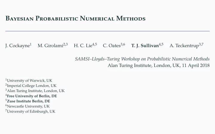
Bayesian Probabilistic Numerical Methods J. Cockayne 1 - PowerPoint PPT Presentation
Bayesian Probabilistic Numerical Methods J. Cockayne 1 SAMSILloydsTuring Workshop on Probabilistic Numerical Methods Alan Turing Institute, London, UK, 11 April 2018 1 University of Warwick, UK 2 Imperial College London, UK 3 Alan Turing
Bayesian Probabilistic Numerical Methods J. Cockayne 1 SAMSI–Lloyds–Turing Workshop on Probabilistic Numerical Methods Alan Turing Institute, London, UK, 11 April 2018 1 University of Warwick, UK 2 Imperial College London, UK 3 Alan Turing Institute, London, UK 4 Free University of Berlin, DE 5 Zuse Institute Berlin, DE 6 Newcastle University, UK 7 University of Edinburgh, UK M. Girolami 2 , 3 H. C. Lie 4 , 5 C. Oates 3 , 6 T. J. Sullivan 4 , 5 A. Teckentrup 3 , 7
A Probabilistic Treatment of Numerics? The last 5 years have seen a renewed interest in probabilistic perspectives on defjnitions are needed! To make these ideas precise and to relate them to one another, some concrete Bayesian inverse problems to speak a common statistical language. Accounting for the impact of discretisation error in a statistical way allows forward and nonlinear and evolutionary contexts can be hard ! If discretisation error is not properly accounted for, then biased and over-confjdent “Big data” problems often require (random) subsampling. viewpoint (Traub et al., 1988; Ritter, 2000; Trefethen, 2008)? Worst-case errors are often too pessimistic — perhaps we should adopt an average-case To a statistician’s eye, numerical tasks look like inverse problems. There are many ways to motivate this modelling choice: (1988); Skilling (1992). continuing a theme with a long heritage: Poincaré (1896); Larkin (1970); Diaconis numerical tasks — e.g. quadrature, ODE and PDE solution, optimisation — 2/41 inferences result (Conrad et al., 2016). However, the necessary numerical analysis in
Outline 1. Numerics: An Inference Perspective 2. Bayes’ Theorem via Disintegration 3. Optimal Information 4. Numerical Disintegration 5. Coherent Pipelines of BPNMs 6. Randomised Bayesian Inverse Problems 7. Closing Remarks 3/41
An Inference Perspective on Numerical Tasks
C 0 0 1 t i u t i 0 u t d t t i y i n 1 y i — does not! (cf. O’Hagan, 1987) An Abstract View of Numerical Methods i : they estimate Q x by b A x . N.B. Some methods try to “invert” A , form an estimate of x , then apply Q . i Vanilla Monte Carlo — b 1 1 n n i Conventional numerical methods are cleverly-designed functions b 1 An abstract setting for numerical tasks consists of three spaces and two functions: Q u 1 i m A u m 0 1 Example 1 (Quadrature) 4/41 X , where an unknown/variable object x or u lives; dim X = ∞ A , where we observe information A ( x ) , via a function A : X → A ; dim A < ∞ Q , with a quantity of interest Q : X → Q .
t i y i n 1 y i — does not! (cf. O’Hagan, 1987) An Abstract View of Numerical Methods i Conventional numerical methods are cleverly-designed functions b i n n 1 1 i Vanilla Monte Carlo — b N.B. Some methods try to “invert” A , form an estimate of x , then apply Q . . estimate Q x by b A x : they 4/41 Example 1 (Quadrature) An abstract setting for numerical tasks consists of three spaces and two functions: X , where an unknown/variable object x or u lives; dim X = ∞ A , where we observe information A ( x ) , via a function A : X → A ; dim A < ∞ Q , with a quantity of interest Q : X → Q . X = C 0 ([ 0 , 1 ] ; R ) A = ([ 0 , 1 ] × R ) m Q = R ∫ 1 A ( u ) = ( t i , u ( t i )) m Q ( u ) = 0 u ( t ) d t i = 1
An Abstract View of Numerical Methods i Example 1 (Quadrature) N.B. Some methods try to “invert” A , form an estimate of x , then apply Q . An abstract setting for numerical tasks consists of three spaces and two functions: 4/41 X , where an unknown/variable object x or u lives; dim X = ∞ A , where we observe information A ( x ) , via a function A : X → A ; dim A < ∞ Q , with a quantity of interest Q : X → Q . X = C 0 ([ 0 , 1 ] ; R ) A = ([ 0 , 1 ] × R ) m Q = R ∫ 1 A ( u ) = ( t i , u ( t i )) m Q ( u ) = 0 u ( t ) d t i = 1 Conventional numerical methods are cleverly-designed functions b : A → Q : they estimate Q ( x ) by b ( A ( x )) . Vanilla Monte Carlo — b (( t i , y i ) n i = 1 ) : = 1 n ∑ n i = 1 y i — does not! (cf. O’Hagan, 1987)
An Abstract View of Numerical Methods ii Question: What makes for a “good” numerical method? (Larkin, 1970) The worst-case error : this Bayesian solution always well-defjned, and what are its error properties? 5/41 Answer 1, Gauss: b ◦ A = Q on a “large” fjnite-dimensional subspace of X . Answer 2, Sard (1949): b ◦ A − Q is “small” on X . In what sense? e WC : = sup ∥ b ( A ( x )) − Q ( x ) ∥ Q . x ∈X The average-case error with respect to a probability measure µ on X : ∫ e AC : = X ∥ b ( A ( x )) − Q ( x ) ∥ Q µ ( d x ) . To a Bayesian , seeing the additional structure of µ , there is “only one way forward”: if x ∼ µ , then b ( A ( x )) should be obtained by conditioning µ and then applying Q . But is
Rev. Bayes Does Some Numerics i A � Q � 6/41 X A Q
Rev. Bayes Does Some Numerics i � � � � � � � � � � � � � � b � Q � A 6/41 X A Q b : A → Q
Rev. Bayes Does Some Numerics i � � � � Probabilistic! Go � � � � � � � � b A � Q � � � � � � 6/41 A # P X P A X A δ Q # P Q A Q b : A → Q
Rev. Bayes Does Some Numerics i � Probabilistic! � � � � � � � � � � � � � � � � Go 6/41 � � � � � � � � b � � Q � � � � A � A # P X P A X A δ Q # P Q A Q a �→ B ( µ , a ) B : P X × A → P Q b : A → Q
Rev. Bayes Does Some Numerics i � � � � � � � � � � � � � � � Example 2 (Quadrature) A deterministic numerical method uses only the spaces and data to produce a point estimate of the integral. A probabilistic numerical method converts an additional belief about the integrand into a belief about the integral. � 6/41 Probabilistic! � A � Q � b � � � � � � � � � � � � � Go A # P X P A X A δ Q # P Q A Q a �→ B ( µ , a ) B : P X × A → P Q b : A → Q X = C 0 ([ 0 , 1 ] ; R ) A = ([ 0 , 1 ] × R ) m Q = R ∫ 1 A ( u ) = ( t i , u ( t i )) m Q ( u ) = 0 u ( t ) d t i = 1
Rev. Bayes Does Some Numerics i � � ‘Bayes’ � ✤ � � � � � � Go � � � � � � Defjnition 2 (Bayesian PNM) through Q : Zellner (1988) calls B an “information processing rule”. Probabilistic! 6/41 � b � � � � � � � � � � Q � � � � A � A # ❣ P X P A X A ❲ � ◆ ◆ ◆ ◆ ◆ ◆ ◆ a �→ µ a δ Q # P Q A Q a �→ B ( µ , a ) B : P X × A → P Q b : A → Q A PNM B ( µ , · ) : A → P Q with prior µ ∈ P X is Bayesian for a quantity of interest Q : X → Q and information operator A : X → A if the bottom-left A - P X - P Q triangle commutes, i.e. the output of B is the push-forward of the conditional distribution µ a B ( µ , a ) = Q # µ a , for A # µ -almost all a ∈ A .
C 0 0 1 / MAP estimator for the defjnite integral is the trapezoidal rule, i.e. integration using Rev. Bayes Does Some Numerics ii Defjnition 3 (Bayesian PNM) Example 4 Under the Gaussian Brownian motion prior on , the posterior mean linear interpolation (Sul din, 1959, 1960). The integrated Brownian motion prior corresponds to integration using cubic spline interpolation. 7/41 A PNM B with prior µ ∈ P X is Bayesian for a quantity of interest Q and information A if its output is the push-forward of the conditional distribution µ a through Q : for A # µ -almost all a ∈ A . B ( µ , a ) = Q # µ a ,
Rev. Bayes Does Some Numerics ii Defjnition 3 (Bayesian PNM) Example 4 The integrated Brownian motion prior corresponds to integration using cubic spline interpolation. 7/41 A PNM B with prior µ ∈ P X is Bayesian for a quantity of interest Q and information A if its output is the push-forward of the conditional distribution µ a through Q : for A # µ -almost all a ∈ A . B ( µ , a ) = Q # µ a , Under the Gaussian Brownian motion prior on X = C 0 ([ 0 , 1 ] ; R ) , the posterior mean / MAP estimator for the defjnite integral is the trapezoidal rule, i.e. integration using linear interpolation (Sul ′ din, 1959, 1960).
A Rogue’s Gallery of Bayesian and non-Bayesian PNMs 8/41
Generalising Bayes’ Theorem via Disintegration
Bayes’ Theorem Thus, we are expressing PNMs in terms of Bayesian inverse problems (Stuart, 2010). But a naïve interpretation of Bayes’ rule makes no sense here, because While linear-algebraic tricks work for linear conditioning of Gaussians, in general we 9/41 supp ( µ a ) ⊆ X a : = { x ∈ X | A ( x ) = a } , typically µ ( X a ) = 0, and — in contrast to typical statistical inverse problems — we think of the observation process as noiseless. E.g. quadrature example from earlier, with A ( u ) = ( t i , u ( t i )) m i = 1 . Thus, we cannot take the usual approach of defjning µ a via its prior density as d µ a d µ ( x ) ∝ likelihood ( x | a ) because this density “wants” to be the indicator function 1 [ x ∈ X a ] . condition on events of measure zero using disintegration.
Recommend
More recommend
Explore More Topics
Stay informed with curated content and fresh updates.
