Bayesian Networks 2 Recap of last lecture: Modeling causal - PDF document

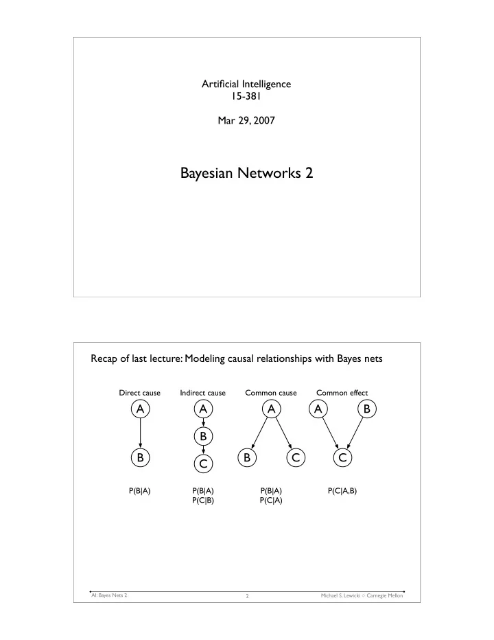
Artificial Intelligence 15-381 Mar 29, 2007 Bayesian Networks 2 Recap of last lecture: Modeling causal relationships with Bayes nets Direct cause Indirect cause Common cause Common effect A A A A B B B B C C C P(B|A) P(B|A) P(B|A) P(C|A,B) P(C|B) P(C|A) AI: Bayes Nets 2 Michael S. Lewicki � Carnegie Mellon 2

Recap (cont’d) W B P(O|W,B) F F 0.01 F T 0.25 P(W) T F 0.05 P(B) 0.05 T T 0.75 0.001 wife burglar W P(C|W) B P(D|B) F 0.01 F 0.001 T 0.95 T 0.5 car in garage open door damaged door • The structure of this model allows a simple expression for the joint probability P ( x 1 , . . . , x n ) ≡ P ( X 1 = x 1 ∧ . . . ∧ X n = x n ) n � = P ( x i | parents( X i )) i =1 ⇒ P ( o, c, d, w, b ) = P ( c | w ) P ( o | w, b ) P ( d | b ) P ( w ) P ( b ) AI: Bayes Nets 2 Michael S. Lewicki � Carnegie Mellon 3 Recall how we calculated the joint probability on the burglar network: • P(o,w,¬b,c,¬d) = P(o|w,¬b)P(c|w)P(¬d|¬b)P(w)P(¬b) = 0.05 � 0.95 � 0.999 � 0.05 � 0.999 = 0.0024 • How do we calculate P(b|o), i.e. the probability of a burglar given we see the open door? • This is not an entry in the joint distribution. W B P(O|W,B) F F 0.01 F T 0.25 P(W) T F 0.05 P(B) 0.05 T T 0.75 0.001 wife burglar W P(C|W) B P(D|B) F 0.01 F 0.001 T 0.95 T 0.5 car in garage open door damaged door AI: Bayes Nets 2 Michael S. Lewicki � Carnegie Mellon 4

Computing probabilities of propositions • How do we compute P(o|b)? - Bayes rule - marginalize joint distribution AI: Bayes Nets 2 Michael S. Lewicki � Carnegie Mellon 5 Variable elimination on the burglary network • As we mentioned in the last lecture, we could do straight summation: p ( b | o ) = α p ( o, w, b, c, d ) � = α p ( o | w, b ) p ( c | w ) p ( d | b ) p ( w ) p ( b ) w,c,d • But: the number of terms in the sum is exponential in the non-evidence variables. • This is bad, and we can do much better. • We start by observing that we can pull out many terms from the summation. AI: Bayes Nets 2 Michael S. Lewicki � Carnegie Mellon 6

Variable elimination • When we’ve pulled out all the redundant terms we get: � � � p ( b | o ) = α p ( b ) p ( d | b ) p ( w ) p ( o | w, b ) p ( c | w ) w c d • We can also note the last term sums to one. In fact, every variable that is not an ancestor of a query variable or evidence variable is irrelevant to the query, so we get � � p ( b | o ) = α p ( b ) p ( d | b ) p ( w ) p ( o | w, b ) w d which contains far fewer terms: In general, complexity is linear in the # of CPT entries. • This method is called variable elimination . - if # of parents is bounded, also linear in the number of nodes. - the expressions are evaluated in right-to-left order (bottom-up in the network) - intermediate results are stored - sums over each are done only for those expressions that depend on the variable • Note: for multiply connected networks, variable elimination can have exponential complexity in the worst case. • This is similar to CSPs, where the complexity was bounded by the hypertree width. AI: Bayes Nets 2 Michael S. Lewicki � Carnegie Mellon 7 Inference in Bayesian networks • For queries in Bayesian networks, we divide variables into three classes: - evidence variables: e = {e 1 , . . . , e m } what you know - query variables: x = {x 1 , . . . , x n } what you want to know - non-evidence variables: y = {y 1 , . . . , y l } what you don’t care about • The complete set of variables in the network is {e ∪ x ∪ y}. • Inferences in Bayesian networks consist of computing p(x|e), the posterior probability of the query given the evidence: p ( x | e ) = p ( x, e ) � = α p ( x, e ) = α p ( x, e, y ) p ( e ) y • This computes the marginal distribution p(x,e) by suming the joint over all values of y. • Recall that the joint distribution is defined by the product of the conditional pdfs: � p ( z ) = P ( z i | parents( z i )) i =1 where the product is taken over all variables in the network. AI: Bayes Nets 2 Michael S. Lewicki � Carnegie Mellon 8

The generalized distributive law • The variable elimination algorithm is an instance of the generalized distributive law. • This is the basis for many common algorithms including: - the fast Fourier transform (FFT) - the Viterbi algorithm (for computing the optimal state sequence in an HMM) - the Baum-Welch algorithm (for computing the optimal parameters in an HMM) • We’ll come back to some of these in a future lecture AI: Bayes Nets 2 Michael S. Lewicki � Carnegie Mellon 9 Clustering algorithms • Inference is efficient if you have a polytree , ie a singly connected network. • But what if you don’t? • Idea: Convert a non-singly connected network to an equivalent singly connected network. Cloudy ?? Sprinkler Rain ?? Wet Grass ?? What should go into the nodes? AI: Bayes Nets 2 Michael S. Lewicki � Carnegie Mellon 10

Clustering or join tree algorithms Idea: merge multiply connected nodes into a single, higher- P(C) P(C) dimensional case. 0.50 0.50 Cloudy Cloudy P(S+R=x|C) C TT TF FT FF Sprinkler Rain Spr+Rain T .08 .02 .72 .18 F .10 .40 .10 .40 C P(S|C) C P(R|C) T 0.10 T 0.80 Wet Grass Wet Grass F 0.50 F 0.20 S R P(W|S,R) S+R P(W|S+R) T T 0.99 T T 0.99 Can take exponential T F 0.90 T F 0.90 time to construct CPTs F T 0.90 F T 0.90 But approximate F F 0.01 F F 0.01 algorithms usu. give reasonable solutions. AI: Bayes Nets 2 Michael S. Lewicki � Carnegie Mellon 11 Example: Pathfinder Pathfinder system. (Heckerman, Probabilistic Similarity Networks, MIT Press, Cambridge MA). • Diagnostic system for lymph-node diseases. • 60 diseases and 100 symptoms and test-results. • 14,000 probabilities. • Expert consulted to make net. • 8 hours to determine variables. • 35 hours for net topology. • 40 hours for probability table values. • Apparently, the experts found it quite easy to invent the causal links and probabilities. Pathfinder is now outperforming the world experts in diagnosis. Being extended to several dozen other medical domains. AI: Bayes Nets 2 Michael S. Lewicki � Carnegie Mellon 12

Another approach: Inference by stochastic simulation Basic idea: 1. Draw N samples from a sampling distribution S 2. Compute an approximate posterior probability 3. Show this converges to the true probability AI: Bayes Nets 2 Michael S. Lewicki � Carnegie Mellon 13 Sampling with no evidence (from the prior) function Prior-Sample ( bn ) returns an event sampled from bn inputs : bn , a belief network specifying joint distribution P ( X 1 , . . . , X n ) x ← an event with n elements for i = 1 to n do x i ← a random sample from P ( X i | parents ( X i )) given the values of Parents ( X i ) in x return x (the following slide series is from our textbook authors.) AI: Bayes Nets 2 Michael S. Lewicki � Carnegie Mellon 14

P(C) .50 Cloudy C P(S|C) C P(R|C) Rain Sprinkler T .10 T .80 F .50 F .20 Wet Grass S R P(W|S,R) T T .99 T F .90 F T .90 F F .01 AI: Bayes Nets 2 Michael S. Lewicki � Carnegie Mellon 15 P(C) .50 Cloudy C P(S|C) C P(R|C) Rain Sprinkler T .10 T .80 F .50 F .20 Wet Grass S R P(W|S,R) T T .99 T F .90 F T .90 F F .01 AI: Bayes Nets 2 Michael S. Lewicki � Carnegie Mellon 16

P(C) .50 Cloudy C P(S|C) C P(R|C) Rain Sprinkler T .10 T .80 F .50 F .20 Wet Grass S R P(W|S,R) T T .99 T F .90 F T .90 F F .01 AI: Bayes Nets 2 Michael S. Lewicki � Carnegie Mellon 17 P(C) .50 Cloudy C P(S|C) C P(R|C) Rain Sprinkler T .10 T .80 F .50 F .20 Wet Grass S R P(W|S,R) T T .99 T F .90 F T .90 F F .01 AI: Bayes Nets 2 Michael S. Lewicki � Carnegie Mellon 18

P(C) .50 Cloudy C P(S|C) C P(R|C) Rain Sprinkler T .10 T .80 F .50 F .20 Wet Grass S R P(W|S,R) T T .99 T F .90 F T .90 F F .01 AI: Bayes Nets 2 Michael S. Lewicki � Carnegie Mellon 19 P(C) .50 Cloudy C P(S|C) C P(R|C) Rain Sprinkler T .10 T .80 F .50 F .20 Wet Grass S R P(W|S,R) T T .99 T F .90 F T .90 F F .01 AI: Bayes Nets 2 Michael S. Lewicki � Carnegie Mellon 20

P(C) .50 Cloudy C P(S|C) C P(R|C) Rain Sprinkler T .10 T .80 F .50 F .20 Wet Grass S R P(W|S,R) T T .99 T F .90 F T .90 Keep sampling to estimate joint F F .01 probabilities of interest. AI: Bayes Nets 2 Michael S. Lewicki � Carnegie Mellon 21 What if we do have some evidence? Rejection sampling. ˆ P ( X | e ) estimated from samples agreeing with e function Rejection-Sampling ( X , e , bn , N ) returns an estimate of P ( X | e ) local variables : N , a vector of counts over X , initially zero for j = 1 to N do x ← Prior-Sample ( bn ) if x is consistent with e then N [ x ] ← N [ x ]+1 where x is the value of X in x return Normalize ( N [ X ]) E.g., estimate P ( Rain | Sprinkler = true ) using 100 samples 27 samples have Sprinkler = true Of these, 8 have Rain = true and 19 have Rain = false . ˆ P ( Rain | Sprinkler = true ) = Normalize ( � 8 , 19 � ) = � 0 . 296 , 0 . 704 � Similar to a basic real-world empirical estimation procedure AI: Bayes Nets 2 Michael S. Lewicki � Carnegie Mellon 22