Bayesian method probabilities Application of Bayesian methods - PDF document
N. Salamin c Sept 2007 Lecture outline Bayesian setting Definition Simple example Phylogeny and bioinformatics for evolution MCMC Normalizing constant MCMC in practice Proposal distribution Prior distribution Posterior Bayesian
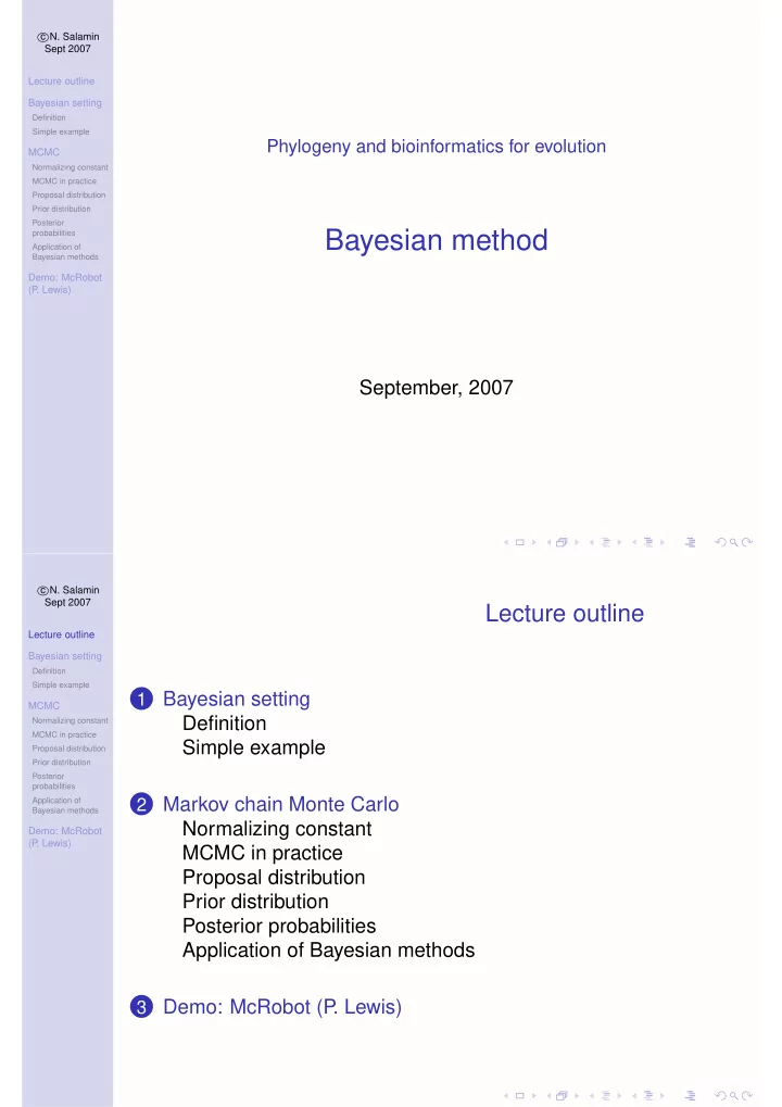
� N. Salamin c Sept 2007 Lecture outline Bayesian setting Definition Simple example Phylogeny and bioinformatics for evolution MCMC Normalizing constant MCMC in practice Proposal distribution Prior distribution Posterior Bayesian method probabilities Application of Bayesian methods Demo: McRobot (P . Lewis) September, 2007 � N. Salamin c Sept 2007 Lecture outline Lecture outline Bayesian setting Definition Simple example Bayesian setting 1 MCMC Definition Normalizing constant MCMC in practice Simple example Proposal distribution Prior distribution Posterior probabilities Markov chain Monte Carlo Application of 2 Bayesian methods Normalizing constant Demo: McRobot (P . Lewis) MCMC in practice Proposal distribution Prior distribution Posterior probabilities Application of Bayesian methods Demo: McRobot (P . Lewis) 3
� N. Salamin c Sept 2007 Lecture outline Lecture outline Bayesian setting Definition Simple example Bayesian setting 1 MCMC Definition Normalizing constant MCMC in practice Simple example Proposal distribution Prior distribution Posterior probabilities Markov chain Monte Carlo Application of 2 Bayesian methods Normalizing constant Demo: McRobot (P . Lewis) MCMC in practice Proposal distribution Prior distribution Posterior probabilities Application of Bayesian methods Demo: McRobot (P . Lewis) 3 � N. Salamin c Sept 2007 Bayesian methods Lecture outline Bayesian setting The likelihood calculation is used as well by Bayesian methods. Definition Simple example However, another component is added to the method: the prior MCMC distributions. Normalizing constant MCMC in practice Proposal distribution Before observing any data, each parameter will be assigned a Prior distribution Posterior prior distribution probabilities Application of Bayesian methods • topologies Demo: McRobot • branch lengths (P . Lewis) • each parameter of the model of evolution The prior distributions are then combined with the likelihood of the data to give the posterior distribution. This is a highly attractive quantity because it computes what we most need: the probabilities of different hypotheses in the light of the data.
� N. Salamin c Sept 2007 Bayes theorem Lecture outline Bayesian setting Definition Simple example To combine all this together, we use the Bayes theorem MCMC Normalizing constant Prob ( T | D ) = Prob ( T ∪ D ) MCMC in practice Proposal distribution Prob ( D ) Prior distribution Posterior probabilities Application of Bayesian methods Demo: McRobot where Prob ( T ∪ D ) = Prob ( T ) Prob ( D | T ) (P . Lewis) so that Prob ( T | D ) = Prob ( T ) Prob ( D | T ) Prob ( D ) � N. Salamin c Sept 2007 Normalizing constant Lecture outline Bayesian setting The denominator Prob ( D ) is the sum of the numerator Definition Simple example Prob ( T ) Prob ( D | T ) over all possible trees T . MCMC Normalizing constant This quantity is needed to normalize the probabilities of all T so MCMC in practice Proposal distribution Prior distribution that they add up to 1. Posterior probabilities Application of This leads to Bayesian methods Demo: McRobot Prob ( T ) Prob ( D | T ) (P . Lewis) Prob ( T | D ) = T Prob ( T ) Prob ( D | T ) � In words: posterior probability = prior probability × likelihood normalizing constant
� N. Salamin c Sept 2007 Odds ratio Lecture outline Bayesian setting Definition Simple example Bayes theorem can be put in the form of odds-ratio, which is the MCMC odds favoring one hypothesis over another Normalizing constant MCMC in practice Proposal distribution • odds a person has initially (the prior odds) Prior distribution Posterior • multiplied by likelihood ratio under the data probabilities Application of Bayesian methods Demo: McRobot • suppose we favor, in advance, T 1 over T 2 with odds 3 : 2 (P . Lewis) • some data gives Prob ( D | T 1 ) / Prob ( D | T 2 ) = 1 / 2 • data say that T 1 is half as probable than T 2 • posterior odds ratio ( 3 / 2 ) × ( 1 / 2 ) = 3 / 4 After looking at the data, we favor T 2 over T 1 by a factor of 4 : 3 � N. Salamin c Sept 2007 Coin toss Lecture outline Bayesian setting Definition Simple example We want to estimate p , the probability of obtaining head, by MCMC tossing a coin n times, which results in n h heads and n t tails Normalizing constant MCMC in practice Proposal distribution Prior distribution • binomial distribution to calculate the likelihood of p Posterior probabilities Application of � n Bayesian methods � Demo: McRobot p n h ( 1 − p ) n − n h B ( n , n h , p ) = (P . Lewis) n h • we make two trials of 10 and 1000 draws resulting in • 3 heads and 7 tails • 300 heads and 700 tails
Exponential prior � N. Salamin c Sept 2007 Exponential prior Lecture outline 10 tosses Bayesian setting Definition Simple example MCMC Normalizing constant MCMC in practice Proposal distribution Prior distribution Posterior probabilities Application of Bayesian methods Demo: McRobot (P . Lewis) Likelihood 10 coins Posterior 10 coins Exponential prior � N. Salamin c Sept 2007 Exponential prior Lecture outline 1000 tosses Bayesian setting Definition Simple example MCMC Normalizing constant MCMC in practice Proposal distribution Prior distribution Posterior probabilities Application of Bayesian methods Demo: McRobot (P . Lewis) Likelihood 1000 coins Posterior 1000 coins
Exponential prior � N. Salamin c Sept 2007 Flat prior Lecture outline 10 tosses Bayesian setting Definition Simple example MCMC Normalizing constant MCMC in practice Proposal distribution Prior distribution Posterior probabilities Application of Bayesian methods Demo: McRobot (P . Lewis) Likelihood 10 coins Posterior 10 coins Exponential prior � N. Salamin c Sept 2007 Flat prior Lecture outline 1000 tosses Bayesian setting Definition Simple example MCMC Normalizing constant MCMC in practice Proposal distribution Prior distribution Posterior probabilities Application of Bayesian methods Demo: McRobot (P . Lewis) Likelihood 1000 coins Posterior 1000 coins
� N. Salamin c Sept 2007 Lecture outline Lecture outline Bayesian setting Definition Simple example Bayesian setting 1 MCMC Definition Normalizing constant MCMC in practice Simple example Proposal distribution Prior distribution Posterior probabilities Markov chain Monte Carlo Application of 2 Bayesian methods Normalizing constant Demo: McRobot (P . Lewis) MCMC in practice Proposal distribution Prior distribution Posterior probabilities Application of Bayesian methods Demo: McRobot (P . Lewis) 3 � N. Salamin c Sept 2007 Estimating normalizing constant Lecture outline Bayesian setting Definition Simple example Posterior distribution expression has a denominator, i.e. MCMC T Prob ( T ) Prob ( D | T ) , that is often impossible to compute. Normalizing constant � MCMC in practice Proposal distribution Prior distribution Posterior probabilities Fortunately, samples from the posterior distribution can be drawn Application of Bayesian methods using a Markov chain that does not need to know the denominator Demo: McRobot (P . Lewis) • draw a random sample from posterior distribution of trees • becomes possible to make probability statements about true tree • e.g. if 96% of the samples from posterior distribution have (human,chimp) as monophyletic group, probability of this group is 96%
� N. Salamin c Sept 2007 Makov chain Monte Carlo Lecture outline Bayesian setting Definition Simple example Idea: to wander randomly through tree space by sampling trees MCMC until we settle down into an equilibrium distribution of trees that Normalizing constant MCMC in practice has the desired distribution, i.e. posterior distribution. Proposal distribution Prior distribution Posterior probabilities • Markov chain: the new proposed tree will depend only on the Application of Bayesian methods previous one Demo: McRobot (P . Lewis) • to reach equilibrium distribution, the Markov chain must be • aperiodic – no cycles should be present in the Markov chain • irreducible – every trees must be accessible from any other tree • probability of proposing T j when we are at T i is the same as probability of proposing T i when we are at T j • the Markov chain has no end � N. Salamin c Sept 2007 MCMC in practice Lecture outline Bayesian setting Metropolis algorithm Definition Simple example • start with a random tree T i MCMC • select a new tree T j by modifying T i in some way Normalizing constant MCMC in practice Proposal distribution • compute Prior distribution Posterior probabilities R = Prob ( T j | D ) Application of Bayesian methods Prob ( T i | D ) Demo: McRobot (P . Lewis) the normalizing constant being the same, this is R = Prob ( T j ) Prob ( D | T j ) Prob ( T i ) Prob ( D | T i ) • if R ≥ 1, accept T j • if R < 1, draw a random number n between [ 0 , 1 ] and accept T j if R > n , otherwise keep T i
Recommend
More recommend
Explore More Topics
Stay informed with curated content and fresh updates.


