Bayesian approach for similarity testing: concepts and examples - PowerPoint PPT Presentation
Note: it is best to view the slides in presentation mode so the animations can be seen. However there are presenter notes below the slides that may also be clarifying. After the presentation there are some supplementary information that may be of
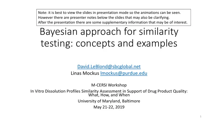
Note: it is best to view the slides in presentation mode so the animations can be seen. However there are presenter notes below the slides that may also be clarifying. After the presentation there are some supplementary information that may be of interest. Bayesian approach for similarity testing: concepts and examples David.LeBlond@sbcglobal.net Linas Mockus lmockus@purdue.edu M-CERSI Workshop In Vitro Dissolution Profiles Similarity Assessment in Support of Drug Product Quality: What, How, and When University of Maryland, Baltimore May 21-22, 2019 1
Acknowledgements to the colleagues who have developed these ideas over the last decade… Yan Shen , Janssen R&D John Peterson, GSK Stan Altan, Janssen R&D Hans Coppenolle, Janssen R&D Areti Manola, Janssen R&D Jyh-Ming Shoung, Janssen R&D Oscar Go , Janssen R&D Linas Mockus, Purdue University Steve Novick, MedImmune … and to YOU !! for your attention, and Harry Yang, MedImmune for considering this approach 2
Some dissolution data: 5 10 15 • Rapidly dissolving Site 1 (Reference) Site 2 (Test) • IV dissolution similarity between 2 100 manufacturing sites • Site 1 (Reference): 8 lots 80 • Site 2 (Test): 5 lots Dissolution (%LC) 60 • Tested in same laboratory • 12 tablets per lot 40 • 5 Time points (minutes): 1, 2, 4, 8, 16 20 • vector 0 5 10 15 Minutes • correlations 3
f 2 (non-Bayesian version) Site 1 (Reference) Site 2 (Test) Minute Mean SD %CV Mean SD %CV 1 3.3 1.6 47.2 5.8 3.2 55.4 2 12.4 4.3 34.6 20.2 6.8 33.5 4 33.4 8.0 23.9 53.7 13.5 25.1 8 71.3 8.7 12.2 80.8 6.0 7.5 16 93.8 2.6 2.7 93.9 3.5 3.7 f 2 = f (Test data, Reference data) f 2 = 38.0 4
The Bayesian answer similarity similarity Question: “My diagnostic test result was X. Do I have the disease?” similarity • Non- Bayesian answer: “Given no disease, the probability of X or worse is P.” similarity • Bayesian answer: “Given X (and other knowledge), the probability of disease is P.” Which answers the question? The Bayesian answer… ICH Q9: “… risk is defined as the combination of • directly addresses the question the probability of occurrence of harm and • quantifies the answer as a probability the severity of that harm ... the protection of the patient by managing the risk to quality • leverages relevant & justifiable prior knowledge should be considered of prime importance.” • is conditional on observed (rather than hypothetical) data 5
* A Bayesian decision tree for in vitro similarity 1. Define similarity parametrically (consider inference space) 2. Model the process that generates data 3. Model prior knowledge 4. Design the demonstration trial (consider inference space) 5. Use MCMC to estimate the posterior probability of similarity ( PPS ) 6. Make a decision If PPS PPS min similar • • Otherwise not similar ____________________________ * More like a telephone pole – no branches 6
1. Define similarity region parametrically (what is the inference space?) Define the comparison: • Test vs Reference? • Test vs some standard of performance? What is similar? Set of all hypothetical: • processes that make lots? • Dissolution profiles, or • lots tested? • Profile differences, or • tablets tested? • Model parameters, or • data results? • Parameter differences, or Define the metric of similarity • Univariate metrics, or • Based on the state of nature we require • … Subset we define as • Not dependent on observed data, similar (Region of experimental design, or analysis Similarity) methodology • Multivariate? • Profile model parameters? • Univariate (e.g., f2)? 7
1. (cont) Candidate similarity regions F 2 = f (true Test quantities, true Reference quantities) 50 Univariate F 2 = f (true Test quantities, fixed Standard quantities) 50 Hyper-rectangle Hyper-ellipsoid Multivariate Allowable ranges for Test – Reference or fixed standard quantities of 3 time points 8
2. Model the process that generates data Site process means (fixed) Observed dissolution profile = Lot to lot deviations … (random multivariate normal) = + + + Tablet to tablet deviations … (random multivariate normal) • For illustration, we will focus on the process mean level Analytical deviations • Inferences at other levels … (random univariate normal) are equally possible 9
2. (cont) Modeling correlations among 5 time points Site 1 Site 2 100 95 100 100 95 100 Observed dissolution profile Shadow of constant 95% 95 95 95 95 16 16 density fitted hyper-ellipse 90 90 90 95 90 95 90 90 70 80 90 70 80 90 80 80 8 8 70 70 70 70 60 60 50 60 70 50 60 70 50 50 80 80 70 50607080 70 50607080 60 60 50 4 50 50 4 50 40 40 30 30 20304050 20304050 20 20 35 35 20253035 20253035 30 30 25 25 2 2 20 20 20 20 15 15 5 101520 10 5 101520 10 5 5 20 20 10 15 20 10 15 20 15 15 1 1 10 10 10 10 5 5 0 5 10 0 5 10 0 0 10 Scatter Plot Matrix
3. Model prior knowledge Prior distributions + - Level Parameters mean Site process mean 5 Population means (fixed) 0.05 density 0.03 0.01 5 SDs Lot to lot deviations 0 10 20 30 40 (random multivariate normal) SD 10 Correlations 0.7 0.6 density 0.5 5 SDs 0.4 Tablet to tablet deviations 0.3 (random multivariate normal) 10 Correlations -1.0 -0.5 0.0 0.5 1.0 Correlation coefficient 4.5 Validation data: 4 Analytical deviations Probability Density 3.5 5 SDs 3 SD = 1.0 based 2.5 (random univariate normal) 2 on 50 df ____________ 1.5 1 0.5 40 parameters 0 0 0.5 1 1.5 2 2.5 Standard Deviation 11
4. Design the demonstration trial (consider inference space) • Time points? • Burden of proof? • H0: Assume similarity unless contradicted by the trial (“difference test”)? • H0: Assume non- similarity unless contradicted by the trial (“equivalence test”)? • Required statistical confidence (probability of incorrectly rejecting H0) and power (probability of correctly rejecting H0)? • Sources and magnitude of variances? • Inter-lot?, Inter-tablet within lot?, analytical? • Number of lots from Test and Reference (unless comparison is to a fixed standard)? • Sampling plan for lots? • Number of tablets from each lot? • Decision metric and its acceptance criterion? ( Bayesian: PPS and PPS min ) 12
5. Use MCMC to estimate PPS MCMC: Simulate Sampling Distribution of data gazillion draws Data from the posterior distribution of Prior distributions of parameters parameters For each draw, Definition of Tally the results to determine whether region of estimate PPS or not similarity similarity criterion is satisfied PPS PPS min ? PPS min Accept similarity Yes No Reject similarity 13
Three illustrations 1. F 2 (Bayesian version), univariate similarity region 2. Hyper-rectangular multivariate similarity region 3. Hyper-ellipsoid multivariate similarity region 14
F 2 (Bayesian version): Estimating PPS Posterior Distribution of F2 MCMC draws from joint posterior 0.08 distribution of process means PPS = 0.06 Probability that Density F 2 50 0.35 0.04 Site 2 process Site 1 process Difference 0.02 F 2 mean (Test) mean (Reference) (Site2 – Site1) Draw 1 2 4 8 16 1 2 4 8 16 1 2 4 8 16 0.00 1 30 40 50 60 70 80 2 F2 … … … … … … … … … … … … … … … … … 15999 Count the fraction of F 2 16000 posterior draws that are 50 15
Hyper-rectangle: Defining similarity Set a fixed similarity range for each time point based on … Shadows of hyper-rectangular similarity region -2 2 6 • Deviations from mean profiles of site 1 clinical lots? • 4 Efficacy/safety considerations (if any)? 1 • -2 Process capability? Tolerance intervals? n-sigma? • Negotiation with regulators? 15 2 • … -5 30 e.g., 4 -10 • Ranges define a Minute Mean Range fixed hyper- 1 3.3 ± 3.2 5 8 rectangular 2 12.4 ± 8.6 -15 similarity region 4 33.4 ± 16.0 • 0 16 0 Applied to all future 8 71.3 ± 17.3 (Test – Reference) -20 -20 16 93.8 ± 5.1 -2 2 6 -5 15 -10 20 -15 5 -20 0 similarity tests. 16
Recommend
More recommend
Explore More Topics
Stay informed with curated content and fresh updates.
