Bank Regulation and Stability: An Examination of the Basel Market - PowerPoint PPT Presentation

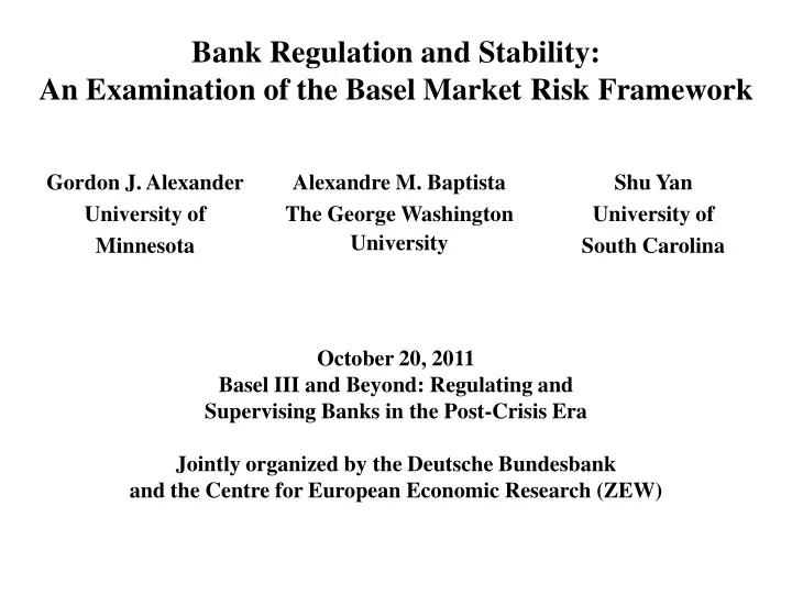
Bank Regulation and Stability: An Examination of the Basel Market Risk Framework Gordon J. Alexander Alexandre M. Baptista Shu Yan University of The George Washington University of University Minnesota South Carolina October 20, 2011 Basel III and Beyond: Regulating and Supervising Banks in the Post-Crisis Era Jointly organized by the Deutsche Bundesbank and the Centre for European Economic Research (ZEW)

1. Motivation • Bank regulators: – Value-at-Risk (VaR) is used to measure the risk in the trading books of large banks and to determine the corresponding minimum capital requirements; – Stress Testing (ST) is used to assess whether banks withstand ‘extreme’ events. • Practitioners: – Banks use VaR and ST to set risk exposure limits (survey of Committee on the Global Financial System, 2005). • Researchers: – VaR is not sub-additive; – VaR does not consider losses beyond VaR; – Advocate Conditional-Value-at-Risk (CVaR): it is sub- additive, and considers losses beyond VaR. • Our paper: – Examines the extent of the conflict between: (1) the popularity of VaR and ST among regulators and practitioners; and (2) the advocacy of CVaR by researchers. – More specifically, we examine the effectiveness of a risk management system based on both VaR and ST constraints in controlling CVaR. – Put differently: is the joint use of VaR and ST ‘equivalent’ to the use of CVaR? 2

2. Main result • The joint use of VaR and ST constraints allows the selection of portfolios with relatively large CVaRs. • Hence, the joint use of VaR and ST constraints is ineffective in controlling CVaR. • This result is consistent with: − Banks around the world suffered sizeable trading losses during the recent crisis. − Trading losses notably exceeded VaR (and even minimum capital requirements). • Our paper supports the view that the Basel market risk framework did not promote bank stability. 3

3. VaR, CVaR, and ST For simplicity, consider a portfolio with a normally distributed return: confidence level 95% Return VaR at the 95% confidence level ( maximum loss under ‘ normal ’ conditions) 4

3. VaR, CVaR, and ST For simplicity, consider a portfolio with a normally distributed return: confidence level 95% Return CVaR = E [ loss | loss ≥ VaR] VaR at the 95% confidence level ( maximum loss under ‘ normal ’ conditions) ( expected loss under ‘ abnormal ’ conditions) 5

3. VaR, CVaR, and ST For simplicity, consider a portfolio with a normally distributed return: confidence level 95% Losses in ST events (e.g., crash of 87 and 9/11) Return CVaR = E [ loss | loss ≥ VaR] VaR at the 95% confidence level ( maximum loss under ‘ normal ’ conditions) ( expected loss under ‘ abnormal ’ conditions) 6

4. Methodology • Allocation problem among nine asset classes: – T-bills (assumed to be risk-free); – Government bonds; – Corporate bonds; and – Six size/value-growth Fama-French portfolios. • Monthly investment horizon; • Historical simulation: – 73% of banks that disclose methodology to estimate VaR report the use of historical simulation (Pérignon and Smith, 2010); – Monthly data during the period 1982–2006; – ST events: (i) 1987 stock market crash; and (ii) 9-11 (CGFS survey, 2005). • Consider three different risk management systems based on: – A single VaR constraint; – Two ST constraints; and – A single VaR constraint and two ST constraints. • Examine whether each set of constraints precludes the selection of all portfolios with relatively large CVaRs; – If a set of constraints precludes such portfolios, it is effective in controlling CVaR; – Otherwise, it is ineffective in controlling CVaR. 7

4. Methodology 1. Choose confidence level α (e.g., 99%) and VaR bound V (e.g., 4%) for the constraint. 8

4. Methodology 1. Choose confidence level α (e.g., 99%) Expected and VaR bound V (e.g., 4%) for the return constraint. E 2. Given the VaR constraint, find maximum feasible expected return E (the minimum expected return E is set to the risk-free return). E CVaR Risk-free return 9

4. Methodology 1. Choose confidence level α (e.g., 99%) Expected and VaR bound V (e.g., 4%) for the return constraint. E 2. Given the VaR constraint, find maximum feasible expected return E (the minimum expected return E is set to the risk-free return). δ = E − 3. Determine ( ) / 100 . E E CVaR Risk-free return 10

4. Methodology is halfway between and E E E 50 1. Choose confidence level α (e.g., 99%) Expected and VaR bound V (e.g., 4%) for the return constraint. E 100 = E 2. Given the VaR constraint, find maximum feasible expected return E (the minimum expected return E is set to the risk-free return). E 50 δ = E − 3. Determine ( ) / 100 . E 4. Construct grid of expected returns: E 0 = E ; E 1 = E + δ ; ... ; E 100 = . E E 0 = E CVaR Risk-free return 11

4. Methodology is % of the way between and E i i E E 1. Choose confidence level α (e.g., 99%) Expected and VaR bound V (e.g., 4%) for the return constraint. E 100 = E 2. Given the VaR constraint, find maximum feasible expected return E (the minimum expected return E is set to the risk-free return). E i δ = E − 3. Determine ( ) / 100 . E 4. Construct grid of expected returns: E 0 = E ; E 1 = E + δ ; ... ; E 100 = . E E 0 = E CVaR Risk-free return 12

4. Methodology is % of the way between and E i i E E 1. Choose confidence level α (e.g., 99%) Expected and VaR bound V (e.g., 4%) for the return Mean-CVaR frontier constraint. E 100 = E 2. Given the VaR constraint, find maximum feasible expected return E Portfolio with (the minimum expected return E is minimum CVaR set to the risk-free return). A E i δ = E − 3. Determine ( ) / 100 . E 4. Construct grid of expected returns: E 0 = E ; E 1 = E + δ ; ... ; E 100 = . E 5. For each value in this grid E i , find E 0 = E maximum efficiency loss M i . CVaR Risk-free return 13

4. Methodology is % of the way between and E i i E E 1. Choose confidence level α (e.g., 99%) Expected and VaR bound V (e.g., 4%) for the return Mean-CVaR frontier constraint. E 100 = E 2. Given the VaR constraint, find maximum feasible expected return E Portfolio with Portfolio with (the minimum expected return E is minimum CVaR maximum CVaR set to the risk-free return). A B E i δ = E − 3. Determine ( ) / 100 . E 4. Construct grid of expected returns: E 0 = E ; E 1 = E + δ ; ... ; E 100 = . E 5. For each value in this grid E i , find E 0 = E maximum efficiency loss M i . CVaR Risk-free return 14

4. Methodology is % of the way between and E i i E E 1. Choose confidence level α (e.g., 99%) Expected and VaR bound V (e.g., 4%) for the return Mean-CVaR frontier constraint. E 100 = E 2. Given the VaR constraint, find maximum feasible expected return E Portfolio with Portfolio with (the minimum expected return E is minimum CVaR maximum CVaR set to the risk-free return). A B E i δ = E − 3. Determine ( ) / 100 . E Maximum 4. Construct grid of expected returns: efficiency loss M i E 0 = E ; E 1 = E + δ ; ... ; E 100 = . E 5. For each value in this grid E i , find E 0 = E maximum efficiency loss M i . CVaR Risk-free return 15

4. Methodology is % of the way between and E i i E E 1. Choose confidence level α (e.g., 99%) Expected and VaR bound V (e.g., 4%) for the return Mean-CVaR frontier constraint. E 100 = E 2. Given the VaR constraint, find maximum feasible expected return E Portfolio with Portfolio with (the minimum expected return E is minimum CVaR maximum CVaR set to the risk-free return). A B E i δ = E − 3. Determine ( ) / 100 . E Maximum 4. Construct grid of expected returns: efficiency loss M i E 0 = E ; E 1 = E + δ ; ... ; E 100 = . E 5. For each value in this grid E i , find E 0 = E maximum efficiency loss M i . CVaR Risk-free return -> For example, if M i = 3% , then the VaR constraint allows the selection of a portfolio with a CVaR that exceeds the CVaR of the minimum CVaR portfolio by 3% . 16

4. Methodology is % of the way between and E i i E E 1. Choose confidence level α (e.g., 99%) Expected and VaR bound V (e.g., 4%) for the return Mean-CVaR frontier constraint. E 100 = E 2. Given the VaR constraint, find maximum feasible expected return E Portfolio with (the minimum expected return E is minimum CVaR Portfolio with set to the risk-free return). maximum CVaR A E i B δ = E − 3. Determine ( ) / 100 . E Maximum 4. Construct grid of expected returns: efficiency loss M i E 0 = E ; E 1 = E + δ ; ... ; E 100 = . E (small) 5. For each value in this grid E i , find E 0 = E maximum efficiency loss M i . CVaR Risk-free return -> More generally, if maximum efficiency loss M i is relatively small , then the VaR constraint is effective in controlling CVaR when the required expected return is E i . 17