Autotuning (2/2): Specialized code generators Prof. Richard Vuduc - PowerPoint PPT Presentation
Autotuning (2/2): Specialized code generators Prof. Richard Vuduc Georgia Institute of Technology CSE/CS 8803 PNA: Parallel Numerical Algorithms [L.18] Thursday, March 6, 2008 1 Todays sources CS 267 at UCB (Demmel & Yelick) Papers
Autotuning (2/2): Specialized code generators Prof. Richard Vuduc Georgia Institute of Technology CSE/CS 8803 PNA: Parallel Numerical Algorithms [L.18] Thursday, March 6, 2008 1
Today’s sources CS 267 at UCB (Demmel & Yelick) Papers from various autotuning projects PHiPAC, ATLAS, FFTW, SPIRAL, TCE See: Proc. IEEE 2005 special issue on Program Generation, Optimization, and Platform Adaptation Me (for once!) 2
Review: Cache-oblivious algorithms 3
A recursive algorithm for matrix-multiply B 11 B 12 Divide all dimensions in half B 21 B 22 Bilardi, et al .: Use grey-code ordering A 11 A 12 C 11 C 12 A 21 A 22 C 21 C 22 No. of misses, with tall-cache assumption: � � � n 3 � � 8 · Q ( n M 2 ) if n > Q ( n ) = ≤ Θ √ 3 3 n 2 L M otherwise 4
Performance-engineering challenges Outer Control Structure Iterative Recursive Inner Control Structure Recursive Iterative Statement Mini-Kernel Micro-Kernel ATLAS CGw/S ATLAS Unleashed Scalarized / None / Coloring / Belady / Compiler BRILA Compiler BRILA 5
Cache-oblivious stencil computation Theorem [Frigo & Strumpen (ICS 2005)]: d = dimension ⇒ � n d · t � Q ( n, t ; d ) = O 1 M d 10 5 t=0 x=0 8 16 6
Cache-conscious algorithm Source: Datta, et al . (2007) 7
Survey of autotuning 8
Early idea seedlings Polyalgorithms : John R. Rice (1969) “A polyalgorithm for the automatic solution of nonlinear equations” (1976) “The algorithm selection problem” Profiling and feedback-directed compilation (1971) D. Knuth: “An empirical study of FORTRAN programs” (1982) S. Graham, P . Kessler, M. McKusick: gprof (1991) P . Chang, S. Mahlke, W-m. W. Hwu: “Using profile information to assist classic code optimizations” Code generation from high-level representations (1989) J. Johnson, R.W. Johnson, D. Rodriguez, R. Tolimieri: “A methodology for designing, modifying, and implementing Fourier Transform algorithms on various architectures.” (1992) M. Covell, C. Myers, A. Oppenheim: “Computer-aided algorithm design and arrangement” (1992) 9
Why doesn’t the compiler do the dirty work? Why doesn’t the compiler do all of this? Analysis Over-specified dependencies Correctness requirements Limited access to relevant run-time information Architecture: Realistic hardware models? Engineering: Hard to modify a production compiler 10
Source: Voss, ADAPT compiler project: http://www.eecg.toronto.edu/~voss/AdaptPage/results.html 11
Source: Voss, ADAPT compiler project: http://www.eecg.toronto.edu/~voss/AdaptPage/results.html 12
Source: Voss, ADAPT compiler project: http://www.eecg.toronto.edu/~voss/AdaptPage/results.html 13
Automatic performance tuning, or “autotuning” Two-phase methodology for producing automatically tuned code Given: Computational kernel or program; inputs; machine Identify and generate a parameterized space of candidate implementations Select the fastest one using empirical modeling and automated experiments “Autotuner” = System that implements this Usually domain-specific (exception: “autotuning/iterative compilers”) Leverage back-end compiler for performance and portability 14
How an autotuner differs from a compiler (roughly) Compiler Autotuner General-purpose Input Specification source code Code generation User responsive Long, but amortized time Static analysis; Automated empirical Implementation some run-time models and selection profiling/feedback experiments 15
Example: What a search space looks like Mflop/s k 0 = 1 m 0 n 0 Platform: Sun Ultra IIi 16 double regs 667 Mflop/s peak Unrolled, pipelined inner-kernel Sun cc v5.0 compiler Source: PHiPAC Project at UC Berkeley (1997) 16
17
Dense linear algebra 18
PHiPAC (1997) Portable High-Performance ANSI C [Bilmes, Asanovic, Chin, Demmel (1997)] Coding guidelines: C as high-level assembly language Code generator for multi-level cache- and register-blocked matrix multiply Exhaustive search over all parameters Began as class project which beat the vendor BLAS 19
PHiPAC coding guideline example: Removing false dependencies Use local variables to remove false dependencies False read-after-write hazard a[i] = b[i] + c; a[i+1] = b[i+1] * d; between a[i] and b[i+1] float f1 = b[i]; float f2 = b[i+1]; In C99, may declare a & b unaliased (“restrict” keyword) a[i] = f1 + c; a[i+1] = f2 * d; 20
ATLAS (1998) “Automatically Tuned Linear Algebra Software” — [R.C. Whaley and J. Dongarra (1998)] Overcame PHiPAC shortcomings on x86 platforms Copy optimization, prefetch, alternative schedulings Extended to full BLAS, some LAPACK support ( e.g. , LU) Code generator (written in C, output C w/ inline-assembly) with search Copy optimization prunes much of PHiPAC’s search space “Simple” line searches See: iterative floating-point kernel optimizer (iFKO) work 21
Search vs. modeling Yotov, et al . “Is search really necessary to generate high- performance BLAS?” “Think globally, search locally” Small gaps ⇒ local search Large gaps ⇒ refine model “Unleashed” ⇒ hand-optimized plug-in kernels 22
Signal processing 23
Motivation for performance tuning pseudo Mflop/s Source: J. Johnson (2007), CScADS autotuning workshop 24
FFTW (1997) “Fastest Fourier Transform in the West” [M. Frigo, S. Johnson (1997)] “ Codelet ” generator (in OCaml) Explicit represent a small fixed-size transform by its computation DAG Optimize DAG: Algebraic transformations, constant folding, “DAG transposition” Schedule DAG cache-obliviously and output as C source code Planner : At run-time, determine which codelets to apply Executor : Perform FFT of a particular size using plan Efficient “plug-in” assembly kernels 25
26
27
Cooley-Tukey FFT algorithm N − 1 � x [ j ] · ω − kj x, y ∈ C N y [ k ] DFT N ( x, k ) ≡ ← N j =0 e 2 π √− 1 /N ≡ ω N N ≡ N 1 · N 2 ⇓ 0 ≤ k 1 < N 1 and 0 ≤ k 2 < N 2 N 2 − 1 �� N 1 − 1 � � � � x [ n 1 · N 2 + n 2 ] · ω − k 1 n 1 · ω − k 1 n 2 · ω − k 2 n 2 y [ k 1 + k 2 · N 1 ] ← N 1 N N 2 n 1 n 2 =0 28
Cooley-Tukey FFT algorithm N − 1 � x [ j ] · ω − kj x, y ∈ C N y [ k ] DFT N ( x, k ) ≡ ← N j =0 e 2 π √− 1 /N ≡ ω N N ≡ N 1 · N 2 ⇓ 0 ≤ k 1 < N 1 and 0 ≤ k 2 < N 2 N 2 − 1 �� N 1 − 1 � � � � x [ n 1 · N 2 + n 2 ] · ω − k 1 n 1 · ω − k 1 n 2 · ω − k 2 n 2 y [ k 1 + k 2 · N 1 ] ← N 1 N N 2 n 1 n 2 =0 N 1 -point DFT Twiddle N 2 -point DFT 29
Cooley-Tukey FFT algorithm: Encoding in the codelet generator N − 1 � x [ j ] · ω − kj x, y ∈ C N y [ k ] DFT N ( x, k ) ≡ ← N j =0 N 2 − 1 �� N 1 − 1 � � � � x [ n 1 · N 2 + n 2 ] · ω − k 1 n 1 · ω − k 1 n 2 · ω − k 2 n 2 y [ k 1 + k 2 · N 1 ] ← N 1 N N 2 n 1 n 2 =0 N 1 -point DFT Twiddle N 2 -point DFT let dftgen( N, x ) ≡ fun k → . . . # DFT N ( x, k ) let cooley tukey( N 1 , N 2 , x ) ≡ let ˆ x ≡ fun n 2 , n 1 → x ( n 2 + n 1 · N 2 ) in let G 1 ≡ fun n 2 → dftgen( N 1 , ˆ x ( n 2 , )) in (Functional let W ≡ fun k 1 , n 2 → G 1 ( n 2 , k 1 ) · ω − k 1 n 2 in pseudo-code) N let G 2 ≡ fun k 1 → dftgen( N 2 , W ( k 1 , )) in fun k → G 2 ( k mod N 1 , k div N 1 ) 30
Planner phase Assembles plan using dynamic programming 31
32
G5 P4 33
SPIRAL (1998) Code generator Represent linear transformations as formulas Symbolic algebra + rewrite engine transforms formulas Search using variety of techniques (more later) 34
Source: J. Johnson (2007), CScADS autotuning workshop 35
Source: J. Johnson (2007), CScADS autotuning workshop 36
High-level representations and rewrite rules ω kl � � DFT N ≡ N 0 ≤ k,l<N � � cos (2 l + 1) k π DCT-2 N ≡ 2 N 0 ≤ k,l<N . . . n = k · m : ( DFT k ⊗ I m ) T n m ( I k ⊗ DFT m ) L n = ⇒ DFT n → k n = k · m, gcd( k, m ) = 1 : = P n ( DFT k ⊗ DFT m ) Q n ⇒ DFT n → p is prime : R T = p ( I 1 ⊕ DFT p − 1 D p ( I 1 ⊕ DFT p − 1 ) R p ⇒ DFT p → . . . � � 1 1 DFT 2 → 1 − 1 37
High-level representations expose parallelism X 1 A X 1 X 2 A X 2 ( I 4 ⊗ A ) · = · X 3 A X 3 X 4 A X 4 AX 1 AX 2 = AX 3 AX 4 A applied 4 times independently 38
High-level representations expose parallelism x 1 x 1 �� � � � � a b x 2 a · I 2 b · I 2 x 2 ⊗ I 2 = · · c d x 3 c · I 2 d · I 2 x 3 x 4 x 4 � � � � x 1 x 3 a + b x 2 x 4 = � � � � x 1 x 3 c + d x 2 x 4 SIMD-vectorizable 39
Search in SPIRAL Search over ruletrees, i.e., possible formula expansions Empirical search Exhaustive Random Dynamic programming Evolutionary search Hill climbing Machine learning methods 40
Example: SMP + vectorization results Source: F. Franchetti (2007), CScADS autotuning workshop 41
Administrivia 42
Recommend
More recommend
Explore More Topics
Stay informed with curated content and fresh updates.
