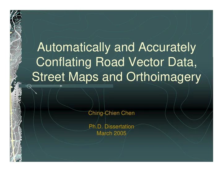
Automatically and Accurately Conflating Road Vector Data, Street - PowerPoint PPT Presentation

Automatically and Accurately Conflating Road Vector Data, Street Maps and Orthoimagery Ching-Chien Chen Ph.D. Dissertation March 2005

Outline Introduction & Motivation Our approach: AMS-conflation Vector and imagery conflation (pre-qualifying research) Map and imagery conflation � Finding control points in the imagery and in the maps � Geospatial point pattern matching (GeoPPM) � Image and map conflation using rubber-sheeting Experimental Results Related Work Conclusion and Future Work

Introduction Geospatial data sources have become widely available Automatically and accurately integrating and aligning two spatial datasets is a challenging problem Street maps Road network Orthoimagery ( in raster format ) ( in vector format ) ( in raster format )

Motivation : Vector and Imagery Integration Challenges Different projections, accuracy levels, resolutions result in spatial inconsistencies Lat / Long Name: Stanley Smith Road Name : Gabriel Dr Address: 125, Gabriel Dr. Range: 20 – 500 Lat / Long City: St. Louis Zip: 63103 State: MO Lat / Long Phone: (314)955-4200 Lat: 38.5943572 Long: -90.4265843 Lat / Long

Motivation : Map and Imagery Integration Lat / Long Lat / Long Lat / Long Integration Challenge � Different geographic projections and accuracy levels Lat / Long

Motivation : Map and Imagery Integration Lat / Long Lat / Long ? Another Integration Challenge Some online maps are not geo-referenced ?

Motivation Traditionally, the problems of vector-imagery and map- imagery alignment have been in the domain of GIS and Computer Vision In GIS literature The alignments were previously performed manually � Commercial products: ESRI MapMerger ; Able R2V ; Intergraph I/RASC In Computer Vision literature The alignments were performed automatically based on image processing techniques � Often required significant CPU time

Outline Introduction & Motivation Our approach: AMS-conflation Vector and imagery conflation (pre-qualifying research) Map and imagery conflation � Finding control points in the imagery and in the maps � Geospatial point pattern matching (GeoPPM) � Image and map conflation using rubber-sheeting Experimental Results Related Work Conclusion and Future Work

Aligning Geospatial Data Using Conflation Technique Conflation: Compiling two geo-spatial datasets by establishing the correspondence between the matched entities and transforming other objects accordingly Requires identifying matched entities, named control points , on both datasets Street map Aligning the Map and Imagery Find Control Points Imagery

Our Approach: AMS-Conflation Automatic Multi-Source Conflation Thesis statement: By exploiting multiple sources of geospatial information, we can achieve automatic and accurate conflation of road vector data, street maps and orthoimagery. Automatically exploiting information from each of the sources to be integrated to generate accurate control point pairs Exploited geospatial information from one data source can help the processing of the other source

AMS-Conflation : Exploit Inferred Information from the Data Source Detected edges Classified road pixels Inferred information from the data source Inferred information Road Intersections from the data source Road Directions • Degree: 3 Detected intersections Detected edges by corner detector • Directions: 1 0 , 90 0 , 180 0 Inferred information from the data source

AMS-Conflation : Exploit Metadata about the Data Source Long: -90.43 10 m Lat: 38.595 Geo-coordinates Resolution 42 m Metadata about the data source Long: -90.42 Lat: 38.594 Metadata about the data source Road widths 153 m Metadata about Resolution the data source (or map scale)

AMS-Conflation : Exploit Peripheral Datasets to the Data Source

AMS-Conflation to Align Vector and Imagery Lat / Long Triangulation and Filtering Rubber-Sheeting Technique Final control points Intermediate control points Control Point Detection Lat / Long Lat / Long Lat / Long

Aligning Vector and Imagery: Finding Control Point Pairs Using Localized Template Matching (LTM) 0.25 On-road Off-road 0.2 0.1 5 0.1 0.05 0 Hue (degree) Bayes Classifier road width and road directions Matching by Correlation

Aligning Vector and Imagery: Filtering Control Point Pairs Using Vector Median Filter (VMF) Y (meter) k% control-point vector Vector median 10 X (meter) O -10 10 -10 W

Completeness : the percentage of the reference roads for which we generated conflated lines Evaluation � (Length of matched reference roads)/(Length of reference roads) Correctness : the percentage of correctly conflated lines with Using road-buffer respect to the total conflated lines method � (Length of matched conflated lines)/(Total length of conflated lines) - Red lines: Reference roads Positional Accuracy : the percentage of conflated roads within x (roadsides) - Blue lines: Reference roads meters to the reference roads (centerlines) Reference roads Reference roads x x x x x x x x x x x x Conflated roads Conflated roads Buffer zone of Buffer zone of buffer width x buffer width x

Results: One of Our Four Test Areas • For the other test areas, we align different road vector data (MO-DOT, NAVSTREETS and TIGER/Lines) with the imagery Yellow Lines: Conflated TIGER/Lines Original Conflated Red Lines: Original TIGER/Lines TIGER/Lines TIGER/Lines Completeness 37.9% 84.7% Correctness 31.3% 88.49% Positional Accuracy

AMS-Conflation to Align Maps and Imagery ? Detect Intersection Map with Unknown Points On the Map Coordinates ? Point Pattern Matching & Map-Imagery Conflation Lat/Long Geo-referenced Points On the Vector-Imagery Imagery Imagery/ Vector Data Conflation Lat/Long

Finding Intersection Points on Maps Difficult to identify intersection points automatically and accurately Varying thickness of lines Single-line map v.s. double-line map Noisy information: symbols and alphanumeric characters We proposed a technique to detect intersections in [acm-gis’04] Our primitive technique is further improved in [Chiang et al.’05 ?] Isolate map data by Remove noisy information by Maps automatic thresholding separating lines and characters and trace parallel lines Apply morphological operator Lines Find Corners Recognize intersections by (using OpenCV) checking line connectivity Detected Points intersections

Finding Intersection Points on Maps Some noisy points will be detected as intersection points. Our geo-spatial point matching algorithm can tolerate the existence of misidentified intersection points. Identify Intersections

Point Pattern Matching Find the mapping between these points Why ? To generate a set of control point pairs How to solve the point sets matching problem : A geometric point sets matching problem Find the transformation T between the layout (with relative distances) of the two point sets 80 points 400 points Example: (lon,lat) = (-118.407088,33.92993) Example: (x,y) = (83,22)

Point Pattern Matching: Finding the Transformation Transformation = Scaling + Translation Scaling in West-East direction Transforms most points on map to points on imagery Find matching point pairs to solve this transformation Scaling in North-South direction

Point Pattern Matching: A Brute-Force Algorithm Iterate all point pair in M, and for each chosen point pair in M examining all point pairs in S Time-consuming : O(m 3 n 2 log n) Can we improve it by randomization ? Not always ! � Noisy points on maps � Some missing points on imagery Check all pairs on S Transformation T ? Transformation T m Points on Map M n Points on Image S Apply T

Geospatial Point Pattern Matching (GeoPPM): Exploit Geometric Info. Associated with Each Intersection Intersection degree: the number of intersected roads Directions of Intersected road segments Degree:3; Directions:0, 90, 270

Geospatial Point Pattern Matching (GeoPPM): Exploit Map Scale We need to consider translation only O(m 3 n 2 log n) � O(m 2 n log n) Point Pattern on Imagery North Transform points to another space based lat/long East West South Point Pattern Matching North Point Pattern on Map based on translation Transform points to another space based on map-scales East West South

Geospatial Point Pattern Matching (GeoPPM): For Map with Unknown Map Scale Exploiting Point Density and Localized Distribution of Points Assumption: we focus on medium to high resolution maps � We are conflating maps with high resolution imagery ! Level 1: 1.2 m/pixel Level 2: 4.25 m/pixel Level 3: 14.08 m/pixel Level 4: 35 m/pixel Coarse level map: map with smaller map-scale (low resolution)

Geospatial Point Pattern Matching (GeoPPM): Exploit Point Density 40 800 55 points 1059 points

Geospatial Point Pattern Matching (GeoPPM): Exploit Localized Distribution of Points The points are in a cluster ! 57 detected map points 1059 points

Geospatial Point Pattern Matching (GeoPPM): Exploit Localized Distribution of Points Using HiGrid Structure Level 0 ( 1 cell ) Level 2 ( 4 cells ) Level 3 ( 16 cells Level 4 ( 64 cells