automatic adaptive quadrature Sanda Adam & Gheorghe Adam - PowerPoint PPT Presentation

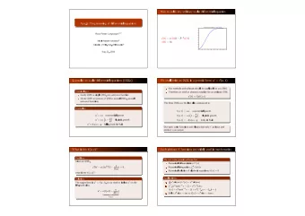
Classes of integrals in the automatic adaptive quadrature Sanda Adam & Gheorghe Adam LIT-JINR Dubna & IFIN-HH Bucharest ROLCG 2016, Bucharest-Magurele, October 26-28, 2016

Overview General frame of the Bayesian automatic adaptive quadrature ( BAAQ )  Three classes of integration domain lengths  Reliability of accuracy specifications  Improved diagnostic tools for Bayesian inference over macroscopic range lengths  Conclusions

General frame (1) The high performance computing in physics research frequently asks for fast and reliable computation of Riemann integrals as part of the models involving evaluation of physical observables. A numerical solution of the Riemann integral 𝑐 𝐽 ≡ 𝐽[𝑔] = 𝑕 𝑦 𝑔 𝑦 𝑒𝑦, −∞ ≤ 𝑏 < 𝑐 ≤ ∞, 𝑏 is sought under the assumption that the real valued integrand function f ( x ) is continuous almost everywhere on [ a, b ] such that I exists and is finite. The weight function 𝑕 𝑦 either absorbs an analytically integrable difficult factor in the integrand (e.g., endpoint singularity or oscillatory function), or else 𝑕 𝑦 ≡ 1, ∀ 𝑦 ∈ 𝑏, 𝑐 .

General frame (2) The automatic adaptive quadrature (AAQ) solution of I provides an approximations 𝑅 ≡ 𝑅 𝑔 to 𝐽 𝑔 based on interpolatory quadrature . The meaningfulness of the output 𝑅 𝑔 is assessed by deriving a bound 𝐹 ≡ 𝐹 𝑔 >0 to the remainder 𝑆 𝑔 = 𝐽 𝑔 − 𝑅 𝑔 . For a prescribed accuracy τ requested at input , the approximation Q to I is assumed to end the computation provided 𝑆 𝑔 < 𝐹 < 𝜐 . The definition of τ needs two parameters: the absolute accuracy 𝜁 𝑏 and the relative accuracy 𝜁 𝑠 , such that 𝜐 = max{𝜁 𝑏 , 𝜁 𝑠 ⋅ |𝐽|} ≃ max{𝜁 𝑏 , 𝜁 𝑠 ⋅ |𝑅|} .

General frame (3) If the condition of termination of the computation is not satisfied, the standard automatic adaptive quadrature (SAAQ) approach to the solution attempts at decreasing the error E by the subdivision of the integration domain [ a, b ] into subranges using bisection and the computation of a local pair { q, e > 0} over each newly defined subrange 𝛽, 𝛾 ⊂ [𝑏, 𝑐] . This procedure builds a subrange binary tree the evolution of which is controlled by an associated priority queue . Local pairs 𝑟 𝑗 , 𝑓 𝑗 > 0 are computed over the i -th subrange of [ a, b ] and global outputs 𝑅 𝑂 , 𝐹 𝑂 > 0 are got by summing the results obtained over the N existing subranges in [ a, b ]. After each subrange binary tree update, the termination criterion is checked until it gets fulfilled.

General frame (4) Within SAAQ, the derivation of practical bounds e > 0 to q rests on probabilistic arguments the validity of which is subject to doubt. The BAAQ advancement to the solution incorporates the rich SAAQ accumulated empirical evidence into a general frame based on the Bayesian inference . While the probabilistic derivation of practical bounds to the local quadrature errors is preserved, each step of the gradual advancement to the solution is scrutinized based on a set of hierarchically ordered criteria which enable decision taking in terms of the stability of the established Bayesian diagnostics. The present report stresses two main things: (i) the need of using length scale dependent quadrature sums and (ii) the importance of the scrutiny of the range of variation of the generated integrand profile in order to decide on the use of a SAAQ-based approach to the solution or on the need of full use of the BAAQ analysis machinery.

Overview  General frame of the Bayesian automatic adaptive quadrature Three classes of integration domain lengths  Reliability of accuracy specifications  Improved diagnostic tools for Bayesian inference over macroscopic range lengths  Conclusions

Symmetric Decomposition of the SAAQ Integrand Profiles •    [ , ] [ , ] a b For any we write the symmetric decomposition                  [ , ] [ , ] [ , ], ( ) / 2 , ( ) / 2 . h • Over the left ( l ) and right ( r ) halves of [ α , β ], the floating point integrand values entering the quadrature sums are computed respectively as         l r ( ), ( ), f f h f f h k k k k where              0 1 , { , } n n n 0 1 CC GK k n stay for the floating point values of the reduced modified quadrature knots associated to either the Clenshaw-Curtis (CC) or the Gauss-Kronrod (GK) quadrature sums. • l = f ( α ), f n r = f ( γ ), f 0 r = f ( β ) are inherited from ancestor Notice that f 0 l = f n subranges while at 0 < η k < 1, values f k l , f k r are computed at each attempt to evaluate I [ α , β ] f. • Definition. The integrand profiles over half-subranges consist of appropriately chosen sets of pairs { η k , f k l } and { η k , f k r } respectively, including those coming from the abscissas pairs { α , γ } and { γ , β }. • Other symmetric quadrature rules result in similarly defined integrand profiles.

Algebraic and Floating Point Degrees of Precision • The algebraic degree of precision , d , is an invariant feature of a quadrature sum over the field ℝ of the real numbers: its value remains constant irrespective of the extent and the localization of the current integration domain over the real axis. • Under floating point computations, the characterization of an interpolatory quadrature sum is made by its floating point degree of precision, d fp . Given the integration domain [ a , b ] ( a ≠ b ), the value of d fp is determined by the magnitude of the parameter ρ = | L | ∕ max{1.0, X }, 0 < ρ ≤ 2, where L = b – a ( L ≠ 0.0); X = max{| a |, | b |} ( X > 0.0). The quantity ρ defines the floating point scale length of [ a , b ].

Features of the Floating Point Degree of Precision • Gliding integration range [0,1] on the real axis. The following plot gives outputs for the family of 1024 integration ranges { [ j α , j α + β ], α = β = 1; j = 0, 1, ..., 1023 } Variation of the floating point degree of precision of the GK 10-21 local quadrature rule over the gliding range [0, 1] versus Gauss-Kronrod 10-21 its distance j from the local quadrature rule origin. It is shown that d fp = d = 31 at low j values ( j = 0, 1, 2), then d fp abruptly decreases at larger but small enough j , to show slower decreasing rates under the displacement of [0,1] far away from the origin, reaching a bottom value d fp = 5 at 701 ≤ j ≤ 1023.

The Inverse Problem • Find the family of the integration ranges 𝛽, 𝛾 over which the floating point degree of precision cannot exceed a prescribed value d . • Possibilities at hand: - d = 2 (the, perhaps composite, trapezoidal rule ), - d = 4 (the, perhaps composite, Simpson rule ), - d ≫ 1 (the SAAQ used GK 10-21 or CC 32 ). Each of these three cases corresponds to specific integration domain lengths, which are separated from each other by two empirically chosen thresholds, 𝜐 𝜈 and 𝜐 𝑛 , defined below. They separate three classes of integration domain lengths corresponding to various quadrature sums at hand.

Three Classes of Finite Integration Domain Lengths • Microscopic ranges [using (composite) trapezoidal rule ( d = 2)], are characterized by the threshold condition 0 < min(𝑌, | L | ∕ X ) ≤ 𝜐 𝜈 = 2 −22 . • Mesoscopic ranges [using (composite) Simpson rule ( d = 4)], are characterized by the threshold condition 𝜐 𝜈 = 2 −22 < min(𝑌, | L | ∕ X ) ≤ 𝜐 𝑛 = 2 −8 . • Macroscopic ranges [using quadrature sums of high algebraic degrees of precision ], are characterized by the threshold condition min(𝑌, | L | ∕ X ) ≤ 𝜐 𝑛 = 2 −8 . == 𝝊 𝝂 = 𝟑 −𝟑𝟑 corresponds to d = 3 == 𝝊 𝒏 = 𝟑 −𝟗 corresponds to d = 8 ; it results in negligible round off over the macroscopic domain lengths.

Exceptional Cases Ending Computation • Irrespective of the domain scale, the early Bayesian assessment of the degree of difficulty of a given integral starts with the symmetrically decomposed integrand profile (IP) generated over the spanning modified reduced quadrature abscissas. A non- commutative decision chain results in the following diagnostics: • (i) The range of the IP variation enables the identification of a constant integrand . • (ii) The measure of oddness of the IP distribution around its centre enables the identification of an odd integrand . • (iii) Splitting the IP into subsets with interlacing abscissas and computation of quadrature sums by composite generalized centroid quadrature sums enables the identification of: - a vanishing integral ; - occurrence of catastrophic cancellation by subtraction ; - occurrence of an easy integral ; - occurrence of a difficult integral asking for Bayesian analysis.