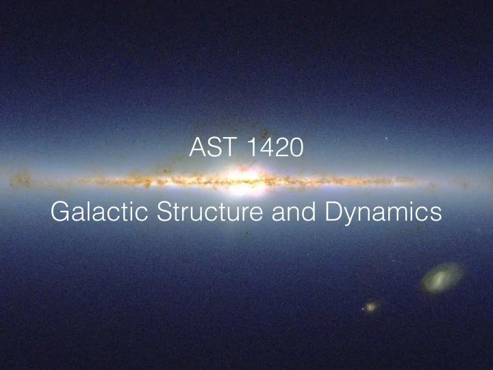
AST 1420 Galactic Structure and Dynamics Third integral Henon - - PowerPoint PPT Presentation

AST 1420 Galactic Structure and Dynamics

Third integral

Henon & Heiles (1964) potential

• Surface of section in (y,vy) at E=1/8

Do all orbits in an axisymmetric potential have a third integral?

No!

• Potentials for which all orbits have a third integral are called

integrable (e.g., the Kuzmin potential)

• Other potentials are non-integrable
• Non-integrable potentials may have large parts of phase

space that are integrable (where orbits have a third integral)

Do all orbits in galactic potentials have a third integral?

• For general galaxies difficult to determine
• Milky Way: solar neighborhood σz =/= σR
• If (E,Lz) were the only

integrals —> σz =/= σR
 because 
 E = 0.5[vR2+vz2]

• Thus, most orbits in the

Milky Way disk must have a third integral

Bovy et al. (2009)

Orbits in triaxial potentials

Orbits in triaxial potentials

• Qualitatively, orbits in

triaxial potentials are similar to those in planar, non- axisymmetric potentials:

• Family of box orbits
• Short-axis tube orbit (~

loop orbits)

• Inner and outer long-axis

tube orbit

• No stable orbit around

the intermediate axis

Statler (1987)

Orbital support for triaxiality

• Box orbits are very important for supporting the triaxiality of the

potential, especially near the center

• Chaos acts to make make the DF more uniform, because the

phase-space density should be ~constant along chaotic trajectories
 —> the velocity dispersion becomes isotropic and thus the support for triaxiality gets destroyed

• Chaos can be induced by central cusp, a central black hole, which

scatter the box orbits when they pass close to the center

• Similarly, growth of axisymmetric disk makes inner galaxy

~axisymmetric —> destroys support for DM box orbits —> DM halo becomes axisymmetric as well

Numerical methods

Today: numerical methods for galactic dynamics

• Numerical methods for simulating stellar and

galactic systems

• Focus solely on gravity, which is the basis of any

simulation code (whether or not it also includes star formation, stellar evolution, gas dynamics, …)

• Technical and algorithmic details are important to

make any code fast—we focus only on basic understanding of numerics

The N body problem

• Numerical simulations of stellar and galactic systems are

known as N-body simulations

• Represent system of stars, dark matter, gas with N bodies

and let them evolve under the force of gravity (+add’l physics)

• Because we typically think of galaxies as being made up of

discrete objects (stars), this makes intuitive sense, but most

• f the mass in galaxies is in (most likely) not this discrete —>

dark matter and gas better described as smooth distributions

• Why does N-body modeling then work?

Galaxies as collisionless systems

• Saying that the gravitational force is smooth is the

same as saying that collisions don’t matter much to the orbits of stars

• To more quantitively determine whether collisions

matter, we can compute the time necessary for close encounters to change the velocity by order unity

• Approximate treatment of galaxies allows a simple

estimate to be made (see notes):

recap

Galaxies as collisionless systems

• Therefore, collisions are only important on

timescales >> the age of the Universe

• We can therefore usefully treat galaxies as smooth

mass distributions

recap

Dense star clusters are collisional systems

• Therefore, collisions in dense star clusters are

important on timescales ~ the age of the Universe

• Dynamics of dense star clusters is much more

complicated!

• Dense star clusters have crossing times of ~1 Myr

and ~105 stars

recap

• Stellar clusters are collisional systems: to simulate their evolution,

we need to take encounters into account —> need to track individual physical bodies (stars in a cluster)

• Galactic systems are collisionless: stars/DM/anything only feels

the smooth gravitational force from the combination of all matter -- > need to track the evolution of the phase-space distribution function f(x,v)

• Clearly two completely different problems!
• Turns out (one) solution to them requires same two steps:
• Compute mutual gravitational force between N bodies
• Integrate orbits numerically under the force of gravity

The N body problem

Some example N- body simulations

Credit: Volker Springel; MPA

Poisson solvers

General methods for obtaining the gravitational potential of a density distribution

• Collisional and collisionless simulations both need to solve the

Poisson equation:

• For a set of N particles for collisional
• For a smooth density for collisionless
• Often smooth density is represented as N discrete spheres and
• btaining the gravitational potential is then similar (but different

considerations on accuracy)

• Methods discussed in class up to now require situations of

some symmetry (spherical, cylindrical razor-thin disk, ellipsoidal, …) —> need more general methods

Basis-function techniques

• Can construct general solutions to the Poisson equation using basis functions
• General idea:
• expand density into sum of contributions for which we know the potential
• total potential is then sum over those contributions
• For general solution, we need sets of basis functions that have the following

properties:

• Complete, orthogonal set of functions that contains all reasonable galactic

densities (smooth, but can be cuspy around the center)

• Simple (analytic) potential for each density basis function (if also
• rthogonal to density functions —> bi-orthogonal)
• Realistic galactic potentials can be expressed using a small number of

basis functions

Basis-function techniques

How to find a basis-function set?

• Many possibilities for basis functions: e.g., functions in 1D
• 1, x, x

2, x 3, …

• Orthogonal polynomials
• sin(x), cos(x), sin(2x), cos(2x), …
• How do you find them? How do you know it’s complete? How do you

pick the right one?

• Solution is to look for eigenfunctions of the Laplace operator ∇

2: functions

f(x) for which ∇

2f(x) = C f(x) similar to eigenvectors

• Eigenfunctions of the Laplacian are automatically orthogonal
• and often clearly form a complete set of functions

How to find eigenfunctions

• f the Laplacian
• Last week we discussed how the Poisson equation separates

into ordinary differential equations for various coordinate systems

• Separation-of-variables also gives a convenient way to search

for eigenfunctions

• We search for eigenfunctions that separate: e.g., in cartesian

coordinates, functions f(x) = X(x) Y(y) Z(z)

• Many galaxies or parts of galaxies are close to spherical —> use

spherical coordinates and search for solutions (not quite eigenfunctions):

Separating the Poisson equation in spherical coordinates

• Plug in solutions, bring phi dependence to right,

everything else left

• Both must be constant, call it m… phi solution:

Separating the Poisson equation in spherical coordinates

• Same procedure for right-hand side: bring theta

dependence to right

• Both sides must be constant = l(l+1); use
• Legendre differential equation —> solved by Legendre

functions of the first kind with integer l (2nd kind and 1st kind with non-integer l diverge at poles)

Separating the Poisson equation in spherical coordinates

• We typically combine the T(theta) and F(phi)

functions into spherical harmonics

• Radial equation becomes
• To find functions that are close to a galactic profile, we

look for solutions of the form

Separating the Poisson equation in spherical coordinates

• If is a realistic galactic potential-density pair,

then the low-order functions are close to galactic

• Radial equation becomes
• Can often be solved analytically: two good cases
• is Plummer (Clutton-Brock 1973)
• is Hernquist (Hernquist & Ostriker 1992)

Basis-function techniques

• Useful for:
• Getting the potential for a more general mass

distribution that is close to spherical (e.g., triaxial halo with changing axis ratios)

• Theoretical investigations of the stability of stellar

systems and the effect of perturbations

• Can also be used to compute the potential for a set of N

particles, automatically smoothing the density (by low-

• rder filtering essentially), but in practice does not work

very well

N-body solvers

N-body solvers

• Problem faced in all N-body simulations: mutual gravity

between N bodies

• 1/|xj-xi| can be softened, but basic problem stands:
• Naive implementations: O(N) / particle x N particles —> O(N2)
• Collisional simulations require high-precision gravity —> directly

compute the sum

• Collisionless simulations can smooth the gravitational field and

use this to speed up code

Softening

• In collisionless N-body simulations, particles are typically softened
• Replace 



 with

• Simple, common softening: point-mass —> Plummer sphere
• Softening removes the unphysical force divergence when ‘particles’

get close

• Doesn’t reduce two-body relaxation much though, just close

encounters

Properties of a good N-body solver

• Good N-body solver depends on context
• Galaxy dynamics:
• Geometry of system often not known a priori (e.g., merger simulation —> where

do the particles end up?)

• Can have range of scales: dynamics in disk (<~ 100 pc) — halo dynamics (100s

kpc), more extreme closer to center

• Want solver that adapts to different geometries and scales
• Star clusters: Geometry typically well-known (e.g., isolated cluster does not move)
• Cosmological structure formation:
• Cosmological box that does not change overall shape much over evolution
• Rather smooth on large scales, periodic boundary conditions
• Range of scales from ‘Universe’ (Gpcs) to individual clusters and galaxies (<~

Mpc)

Direct summation

Direct summation

• Most naive approach: directly compute mutual

gravity using

• Need to determine N(N-1)/2 mutual distances —>

O(N2)

• Straightforward to implement, ‘easy’ to optimize

implementation (incl. hardware)

• Manifestly satisfies Newton’s third law —> conservation of

momentum

Example implementation

(note: inefficient, because we compute all N2 mutual distances

Example implementation

Example implementation

Example implementation

Direct summation

• Method of choice for collisional simulations: star

clusters, particle disks around planets, …

• Currently possible to go to ~N=106 using GPUs
• Not used for collisionless simulations: can use

smoothness of the density field to motivate approximate algorithms

Tree-based gravity solvers

Tree-based gravity solvers

• Introduced by Barnes & Hut (1986; still behind paywall!)
• Use hierarchical tree to divide data set into cells
• Approximate gravitational force by:
• Group distant bodies into large cells
• Group nearby bodies into small cells
• Generally, leads to reduction of O(N) time / force

calculation —> O(ln N)

Hierarchical tree

• Recursively sub-divide data set into smaller and smaller

cells

• For gravity, oct-tree popular choice:
• First level: single cell that covers data in 3D
• Second level: subdivide into eight children, 2 per

dimension

• Third level: subdivide each child into 8 more children
• Stop when cell has <=Nmax bodies (e.g., 1)

Hierarchical tree

Hierarchical tree

Hierarchical tree

Hierarchical tree

Hierarchical tree

Hierarchical tree: 
 real quad-tree example

Hierarchical tree: 
 real quad-tree example

Automatically adapts resolution —> high resolution where there are many particles

Opening angle

• Key to tree-based gravity calculation is approximation of distant

bodies as a single body

• Criterion based on an opening angle
• Cell C with center-of-mass xC spans an angle of θjC when seen from

point xj:

• For point xj all bodies in cell C can be approximated as single body

if the cell appears smaller than a limiting opening angle

• If cell C appears to be larger than the limit, we consider each of its

children and whether they appear to be smaller than θlim, if not, split

Opening angle: example

Opening angle: example

“single-unit cells”

Opening angle: example

“single-unit cells”

Gravity approximation

• To compute the gravity of a given point xj, we

consider all single-unit cells for xj and treat each as a single body (at the center of mass: red square in next slides)

• Typically have O(lnN) single-unit cells —> gravity

calculation takes O(lnN) time / body and O(NlnN) for all bodies

• This is much faster than direct summation

Gravity approximation

Gravity approximation

• Final piece of the puzzle: how to approximate each

cell as a single body

• Simplest: single point-particle with mass = sum of

all masses in cell

• Gravitational potential from cell C is then

Gravity approximation

• Can consider multipole expansion around the

center of mass for higher accuracy (first multipole zero, bc center of mass)

Gravity approximation: example

Tree-based gravity scaling

O(ln N)

Tree-based gravity scaling

Tree setup takes O(N ln N) [~N here]

Fast Multipole Method

• Barnes & Hut tree-based gravity solver uses only the fact

that force from all particles in a distant cell is similar

• Further speed-up possible by using that force on particles

that are close together is similar as well

• Principle of fast-multipole method: expand gravity both

around source (particle acting as source of gravity) and sink (particle on which we want the force) (Greengard & Rokhlin 1987; Dehnen 2002/2002 in astrophysics)

• Leads to O(N) gravity calculation, but more complicated

than Barnes/Hut (larger pre-factor)

Fast Multipole Method

Dehnen & Read (2011)

Particle-mesh technique

Particle-mesh codes

• Quite different approach solves the Poisson equation on

a grid using Fourier transformation

• Poisson equation becomes

~ k2 Φ(~ k) = 4⇡ G ⇢(~ k)

• Easy to solve
• Thus, algorithm becomes
• Assign particles’ mass to grid points (some smoothing)

—> O(N)

• Fourier transform the density —> O( ngrid ln ngrid)
• Solve Poisson above
• Inverse fourier transform the potential —> O( ngrid ln ngrid)

Particle-mesh codes

• Advantages:
• Fast because of fast-fourier-transform techniques
• Ideal for cosmological simulations with periodic boundary

conditions

• Disadvantages:
• Single grid-spacing —> not adaptive to regions of high

density

• Adaptive grids possible (without Fourier), but lead to

energy conservation and issues in non-equilibrium situations

Scaling of collisional and collisions simulations

Numerical orbit integration

Numerical orbit integration

• Motion of body under the force of gravity given by

Newton’s second law or Hamilton’s equations

• Cannot be solved analytically, except in very rare

cases (point-mass, homogeneous sphere, …)

• Thus, need to solve numerically (we have already

done this a lot in the previous weeks)

• Equation is an ordinary differential equation

Numerical orbit integration

• Always solve Hamilton’s equations; system of first-
• rder, linear ordinary differential equations (ODEs)
• Can use any standard ODE solver or specialized

solvers for Hamiltonian systems

General ODE solvers

General ODE solvers

• Equation of motion in cartesian coordinates:
• Or
• Simplest solution: Euler’s method

Euler’s method

Numerical Recipes, Chapter 17

Improving Euler’s method

Numerical Recipes, Chapter 17

Improving Euler’s method

• Use initial derivative to estimate mid-point
• Use derivative at mid-point to advance the full time step
• Example of a Runge-Kutta type method (specifically,

second order Runge-Kutta; RK2)

• Smaller errors than Euler, but two derivative

evaluations

Fourth-order Runge Kutta

• We can build higher-order Runge-Kutta type

methods by using more estimated intermediate points to advance the point by 1 time step

• Coefficients determined by requiring the solution to

be precise up to given order

• Most popular: fourth-order Runge Kutta

Fourth-order Runge Kutta

Numerical Recipes, Chapter 17

Fourth-order Runge Kutta

Higher-order Runge Kutta methods

• We can build even higher-order methods of the same type
• Advantage of some higher orders: can produce multiple

solutions from same set of intermediate points, accurate to different orders

• Can use these multiple solutions to estimate error and use

to adapt the time step —> adaptive time stepping

• Examples: Dormand-Prince methods of order 5 and 8
• RK4 and Dormand-Prince methods are often used in

galactic dynamics

Criticism of standard methods

• Standard methods can give high precision at short

time intervals

• But long-term energy conservation is bad —>

numerical errors build up in every time step

• Useful for few dynamical times (up to hundreds),

but not more (no solar system!)

Hamiltonian integration

Hamiltonian integration

• Standard methods work by approximately solving the

equations for the exact Hamiltonian

• But we could also exactly solve the equations of motion

for an approximate Hamiltonian

• Such methods have the advantage that they exactly

conserve dynamical quantities (phase-space volume, energy, …), but for the wrong system

• If the approximate Hamiltonian is ~ the correct, this

advantage typically leads to great long-term behavior

Discretizing the Hamiltonian

• Let’s work in cartesian coordinates; Hamiltonian
• Hamilton’s equations
• Discretize the Hamiltonian in the following way

with

Discretizing the Hamiltonian

• Discretized Hamiltonian equal to
• Thus, on timescales >> Δt: approximate

Hamiltonian ~ exact Hamiltonian

• Hamilton’s equations for discretized Hamiltonian

Drift-kick

• We can solve the equations of motion as a

combination of drift and kick steps

• From t=ε to t=Δt-ε
• From t=Δt-ε to t=Δt+ε

Drift-kick

• Limit of ε —> 0
• First step: drift
• Second step: kick
• Result similar to Euler, but evaluate force at final point

—> modified Euler, also first-order

Leapfrog integrator

• Simply by shifting by Δt/2, we can build a second-
• rder integrator that only uses a single force evaluation
• This is the drift-kick-drift leapfrog integrator
• Workhorse for collisionless simulations

Advantages of Hamiltonian integration

• Typically have excellent long-term energy

conservation

• Connect to perturbation theory: can split

Hamiltonian into largest contribution + perturbation

• Important in solar-system (and exoplanet)

integrations: can split Hamiltonian into point-mass potentials + small planet-planet perturbations (Wisdom-Holman integrator)

Energy conservation

Bovy (2015)

Conservation of phase- space volume

Bovy (2015)

Individual time steps

• N-body simulations of collisionless systems have wide

range of dynamical timescales

• Use individual time step: particles with short dynamical

times have short time steps, those with long dynamical times have long time steps

• Somewhat unsolved problem of how to best choose

these, standard methods far from optimal

• Most efficient when particles are arranged in hierarchy
• f discrete time steps: block time-step scheme

Block time-step scheme

BT08

and finally….

N-body modeling

N-body modeling

• Now we have the tools to discuss N-body modeling
• Two cases: collisional vs. collisionless
• Collisional: solve evolution of system of N stars under

Hamiltonian

• Collisionless: solve collisionless Boltzmann

equation

Collisional N-body modeling

Collisional N-body modeling

• Need to follow equation of motion under the full Hamiltonian
• Not easy to get around the following procedure:
• Compute all forces using direct summation
• Use numerical integrator to advance orbits
• Typically use more advanced numerical integrators that use

derivatives of the acceleration (+higher!)

• Typically don’t use symplectic integrators for star clusters: need

high precision on short timescales, less important on long

• Need to explicitly deal with close encounters in efficient way

Collisionless N-body modeling

Collisionless N-body modeling

• Coupled equations: collisionless Boltzmann

equation

• Plus Poisson
• Poisson has formal solution

Collisionless N-body modeling

• Solve this system of equations essentially using Liouville’s theorem with

Monte Carlo sample: phase-space density conserved along trajectories

• Monte Carlo sample from initial phase-space DF f(x,v,t=0) with bias

g(x)

• Estimate gravitational potential as Monte-Carlo integral using this

sample

• Integrate each sample’s orbit under this gravitational potential
• Liouville’s theorem means that phase-space density is conserved —>

Monte-Carlo samples remain samples from f(x,v,t=t)