Are marriage-related taxes and Social Security benefits holding back - PowerPoint PPT Presentation

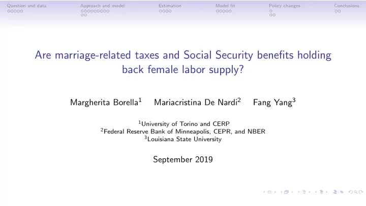
Question and data Approach and model Estimation Model fit Policy changes Conclusions Are marriage-related taxes and Social Security benefits holding back female labor supply? Margherita Borella 1 Mariacristina De Nardi 2 Fang Yang 3 1 University of Torino and CERP 2 Federal Reserve Bank of Minneapolis, CEPR, and NBER 3 Louisiana State University September 2019

Question and data Approach and model Estimation Model fit Policy changes Conclusions U.S. marriage-related policies • Taxes and old age Social Security benefits depend on marital status • Joint income tax • Social Security spousal benefit • Social Security survival benefit

Question and data Approach and model Estimation Model fit Policy changes Conclusions U.S. marriage-related policies • Taxes and old age Social Security benefits depend on marital status • Joint income tax • Social Security spousal benefit • Social Security survival benefit • Question: how do marriage-related policies affect • Labor supply of women • Labor supply of men • Savings • Welfare

Question and data Approach and model Estimation Model fit Policy changes Conclusions U.S. marriage-related policies • Taxes and old age Social Security benefits depend on marital status • Joint income tax • Social Security spousal benefit • Social Security survival benefit • Question: how do marriage-related policies affect • Labor supply of women • Labor supply of men • Savings • Welfare • Labor supply of married women has been changing over time. Do the effects of these policies depend on the cohort? • Two cohorts (1945 cohort and 1955 birth cohorts)

Question and data Approach and model Estimation Model fit Policy changes Conclusions Why might they matter? Marginal tax rate for women Women's marginal tax rates Empirical cumulative distribution 0.3 1 0.9 0.25 0.8 0.2 0.7 Cumulative probability Marginal tax rate 0.15 0.6 0.1 0.5 0.4 0.05 0.3 0 0.2 Married to 75th earner Married to 50th earner -0.05 Married to 25th earner 0.1 Single Women -0.1 0 0 1 2 3 4 5 6 7 8 9 10 -0.2 -0.1 0 0.1 0.2 0.3 Women's income 10 4 Non-working wives' marginal tax rate

Question and data Approach and model Estimation Model fit Policy changes Conclusions Why might they matter? Social Security benefits Social Security Benefit Survivor Benefit 50000 25000 W/ m. benefit W/O m. benefit 45000 20000 Average Wife's Survivor Benefit Average Household Benefit 40000 15000 35000 10000 30000 W/ m. benefit 5000 W/O m. benefit 25000 20000 0 1 2 3 4 5 6 7 8 9 10 1 2 3 4 5 6 7 8 9 10 Wife's own benefit decile Wife's own benefit decile

Question and data Approach and model Estimation Model fit Policy changes Conclusions Participation for women, 1945 and 1955 cohorts Labor Participation 0.9 0.8 0.7 0.6 0.5 Single women, 1945 Married women, 1945 0.4 Single women, 1955 Married women, 1955 0.3 25 30 35 40 45 50 55 60 65 Age Hours

Question and data Approach and model Estimation Model fit Policy changes Conclusions Participation for men, 1945 and 1955 cohorts Labor Participation 1 0.9 0.8 Single men, 1945 Married men, 1945 0.7 Single men, 1955 Married men, 1955 0.6 0.5 0.4 25 30 35 40 45 50 55 60 65 Age Hours

Question and data Approach and model Estimation Model fit Policy changes Conclusions Approach • Partial equilibrium, cohort level analysis

Question and data Approach and model Estimation Model fit Policy changes Conclusions Approach • Partial equilibrium, cohort level analysis • Data • Panel Study of Income Dynamics (PSID): working period • Health and Retirement Study (HRS): retirement period

Question and data Approach and model Estimation Model fit Policy changes Conclusions Approach • Partial equilibrium, cohort level analysis • Data • Panel Study of Income Dynamics (PSID): working period • Health and Retirement Study (HRS): retirement period • Estimate model on each cohort using the Method of Simulated moments (MSM) • Counterfactuals: eliminate marriage-related provisions

Question and data Approach and model Estimation Model fit Policy changes Conclusions Model’s key features • Single and married people • Endogenous human capital • Risks during working period and retirement • Self-insurance: saving and labor supply (hours)

Question and data Approach and model Estimation Model fit Policy changes Conclusions Model’s key features • Single and married people • Endogenous human capital • Risks during working period and retirement • Self-insurance: saving and labor supply (hours) • Government • Taxes married and single people + tax progressivity • Social Security payments (survival and spousal benefits) • Old-age means-tested transfer programs

Question and data Approach and model Estimation Model fit Policy changes Conclusions Model’s key features • Lifecycle model, period length: one year • Working stage ( t 0 =25 to 61) • Alive for sure • Labor productivity shocks • Might get married if single • Risk divorce if married • Both spouses can work

Question and data Approach and model Estimation Model fit Policy changes Conclusions Model’s key features • Lifecycle model, period length: one year • Working stage ( t 0 =25 to 61) • Alive for sure • Labor productivity shocks • Might get married if single • Risk divorce if married • Both spouses can work • Early retirement stage (62 to 65) • Can retire and claim Social Security. Couples retire at the same time. • No marriage and divorce risk

Question and data Approach and model Estimation Model fit Policy changes Conclusions Model’s key features • Lifecycle model, period length: one year • Working stage ( t 0 =25 to 61) • Alive for sure • Labor productivity shocks • Might get married if single • Risk divorce if married • Both spouses can work • Early retirement stage (62 to 65) • Can retire and claim Social Security. Couples retire at the same time. • No marriage and divorce risk • Retirement stage (66 to T =99) • Health shocks • Medical costs • Exogenous probability of death → married people might lose their spouse

Question and data Approach and model Estimation Model fit Policy changes Conclusions Wages • Functions of • Human capital, measured as average past earnings • Wage shocks which follow an AR(1) that depends on gender

Question and data Approach and model Estimation Model fit Policy changes Conclusions Marriage and divorce • Marriage • Probability of marrying: function of age, gender, and wage shock • Conditional on getting married, probability of meeting with a partner with a certain wage shock depends on your wage shock • Conditional partner’s productivity, distribution of partner’s characteristics are assets and human capital • Divorce probability: function of age and wage shocks of both spouses

Question and data Approach and model Estimation Model fit Policy changes Conclusions Children • Exogenous fertility • Number and age structure of children depends on maternal age and marital status • Time costs of raising children • Monetary costs of raising children

Question and data Approach and model Estimation Model fit Policy changes Conclusions Health risks (after age 66) • Age, gender, marital status, and current health affect evolution of • Health • Medical expenses • Survival

Question and data Approach and model Estimation Model fit Policy changes Conclusions Government • Taxes income, progressive taxation of couples and singles t Y − τ i , j T ( Y , i , j , t ) = (1 − λ i , j t ) Y . • Taxes labor income, up to Social Security cap � y t , at rate τ SS to finance old-age t Social Security • Old age means-tested cons. floor c( j ) (Medicaid and SSI)

Question and data Approach and model Estimation Model fit Policy changes Conclusions Household preferences • β = discount factor, i = gender, j = marital status • Time endowment: L i , j = L i , j − n i , j • Leisure l i , j t − φ i , j t I n i , j t t

Question and data Approach and model Estimation Model fit Policy changes Conclusions Household preferences • β = discount factor, i = gender, j = marital status • Time endowment: L i , j = L i , j − n i , j • Leisure l i , j t − φ i , j t I n i , j t t • Singles ) 1 − γ − 1 v ( c t , l t ) = (( c t /η i , j t ) ω l 1 − ω t 1 − γ

Question and data Approach and model Estimation Model fit Policy changes Conclusions Household preferences • β = discount factor, i = gender, j = marital status • Time endowment: L i , j = L i , j − n i , j • Leisure l i , j t − φ i , j t I n i , j t t • Singles ) 1 − γ − 1 v ( c t , l t ) = (( c t /η i , j t ) ω l 1 − ω t 1 − γ • Couples t ) 1 − ω ) 1 − γ − 1 t ) = (( c t /η i , j t ) ω ( l 1 w ( c t , l 1 t , l 2 + 1 − γ (( c t /η i , j t ) 1 − ω ) 1 − γ − 1 t ) ω ( l 2 1 − γ

Question and data Approach and model Estimation Model fit Policy changes Conclusions Value functions for couples and people in couples • Working period • Early retirement • Retirement • People in couples

Question and data Approach and model Estimation Model fit Policy changes Conclusions Value functions for singles • Working period • Early retirement • Retirement