Applications of Bayesian Analysis to Coronal Seismology Iigo - PowerPoint PPT Presentation
Applications of Bayesian Analysis to Coronal Seismology Iigo Arregui True, False, and Uncertain TRUE My name is Iigo Arregui UNCERTAIN But I am happy My name is Harry Warren FALSE to be on his Team! Probability as
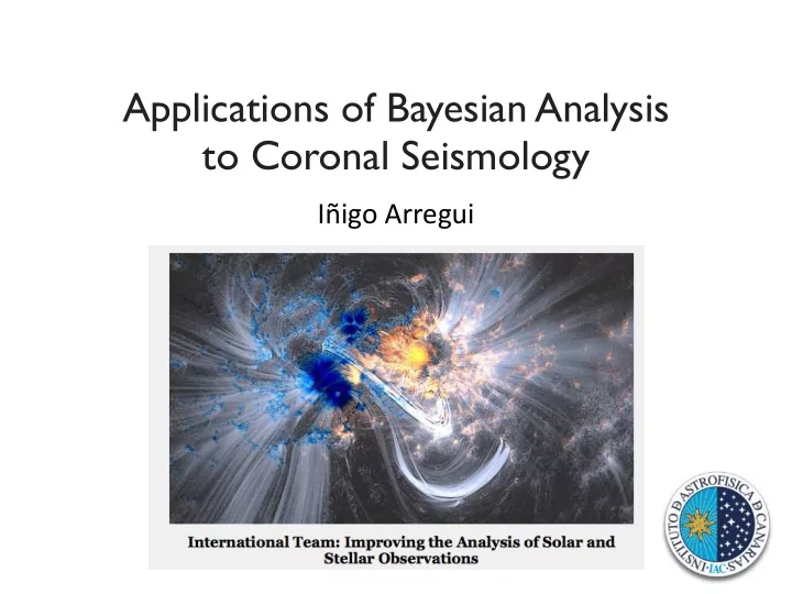
Applications of Bayesian Analysis to Coronal Seismology Iñigo ¡Arregui ¡ ¡
True, False, and Uncertain TRUE My name is Iñigo Arregui UNCERTAIN But I am happy My name is Harry Warren FALSE to be on his Team!
Probability as Extended Logic Logic Probability E. T. Jaynes Aristotle Determines Truth/Falsity Quantifies Uncertainty Outcome: True/False Outcome: Degree of Belief
Seismology of the Solar Atmosphere Aim: determination of difficult to measure physical parameters in e.g.: Coronal loops Prominences Combination of: { - Observations: Wave activity in the solar atmosphere - Theory: MHD wave interpretation
Wave Activity - Observations Rosenberg (70); Trottet+(79) … Aschwanden+(99); Nakariakov+(99); De Pontieu+(07); Okamoto+(07); Cirtain+(07); McIntosh+(11); Kuridze+(13); Morton+(12,13,14);Threlfall+(13); Mathioudakis+(13)… Existence of wave-like dynamics beyond question AR Corona Coronal Loops a n o r o C d e d n e t x E Chromospheric Spicules X-ray Jets Prominence plasmas + chromospheric bright points/mottles + coronal hole structures + filament threads… Time/spatial variation of spectral line properties / imaged emission SST, DST, CoMP, SoHO, TRACE, Hinode, STEREO, SDO, Hi-C, IRIS: increased detail/coverage
Method of MHD Seismology Observations Observations EQUILIBRIUM PARAMETERS OSCILLATIONS (?) Inverse problem Direct problem Theory Theory EQUILIBRIUM MODELS EIGENMODES A well established method to obtain information on properties of the solar atmospheric plasma and field Determination of the magnetic field strength, coronal density scale height, density structuring along and cross coronal loops, etc.
other seismology techniques asteroseismology Geoseismology Helioseismology Magnetoseismology Earth’s interior, earhtquakes and The interior of the Sun Earth’s magnetospheric plasmas related phenomena using sound-gravity waves Disk seismology Tokamaks Neutron star seismology Accretion disks around compact Laboratory/Fusion plasmas objects ?
From classic to Bayesian techniques Confronting observations and theory to infer physical parameters is not an easy task Seismology involves the solution of two different problems Cause Consequences Theoretical Theoretical models Forward problem wave properties and parameters Cause Consequences Observed Unknown physical Inverse problem wave properties conditions/processes Under conditions in which information is incomplete and uncertain We use the rules of probability to make scientific inference and quantify uncertainty
A one-slide introduction to probability What is probability: Probability quantifies randomness and uncertainty What is statistics: Statistics uses probability to make scientific inferences Use of probability: There are two main schools / lines of thought / religions They calculate probabilities of different things! Bayesians Frequentists Measure frequencies Measure informed belief Measure of degree to which a Interpretation Long-run relative frequency in given proposition is supported by of probability the limit of infinite repetitions data Alternative hypotheses: Alternative data: Focus on compare probs. of different compare probs. of different data realizations hypotheses in view of data Counting Useful for Inference and model comparison Characterizing data Astrophysics observational science > data are fixed! The Bayesian framework defines rigorous tools to perform inference and model comparison by looking at how data constrain parameters/models
We cannot state that something is true/false in the solar atmosphere We just try to quantify what to believe And accept that as the best we can do
Bayesian Data Analysis Probabilistic Inference considers the inversion problem as the task of estimating the degree of belief in statements about parameter values/model evidence Bayes’ Rule (Bayes & Price 1763) Posterior p ( θ | D, M ) p ( D | θ , M ) p ( θ | M ) Prior p ( θ | D, M ) = d θ p ( D | θ , M ) p ( θ | M ) , ) p ( θ | M ) � Likelihood function p ( D | θ , M ) | | � � Evidence d θ p ( D | θ , M ) p ( θ | M ) State of knowledge is a combination of what is known a priori independently of data and the likelihood of obtaining a data realisation actually observed as a function of the parameter vector Model Comparison Model Averaging Parameter Inference Compute posterior for different Compare one model Posteriors weighted with combinations of parameters against other model evidence Marginalise Posterior ratios Weighted posterior N Z p ( M j | d ) = p ( d | M i ) p ( M i | d ) p ( M i ) X p ( θ i | d ) = p ( θ | d ) d θ 1 . . . d θ i − 1 d θ i + 1 . . . d θ N . p ( θ | d ) = p ( θ | d, M i ) p ( M i | d ) p ( M j ) . p ( d | M j ) i =1
List of Applications and Methodologies APPLICATIONS Inference of physical parameters in coronal waveguides from observed damped transverse oscillations Inference of cross-field density structure from damped transverse oscillations oscillations Inference of coronal density scale height and coronal magnetic expansion and comparison between stratified and magnetically non-uniform models Model comparison for the density structure along and across coronal waveguides METHODS Markov Chain Monte Carlo sampling of the posterior Computation of marginal posteriors from integrals Computation of marginal likelihood to assess model plausibility Computation of Bayes factors to assess relative model plausibility Computation of weighted posterior to perform model averaging
Example #1 Inference of coronal loop parameters from observations of transverse oscillations
Coronal loop oscillations Aschwanden et al. (1999); Nakariakov et al. (1999); Aschwanden et al. (2002); Schrijver et al. (2002), Verwichte et al. (2004) ... White & Verwichte (2012) Verwichte et al. (2004) Nakariakov et al. (1999) • Transverse standing MHD kink mode of a magnetic flux tube - lateral displacement of the tube Periods ~ 2-11 mins (Nakariakov99)- Multiple harmonics (Verwichte04) Damping times ~ 3-21 mins • Resonant damping - coupling of global motion to local Alfvén waves (Hollweg & Yang88; Goossens02)
Classic inversion - 1D density enhancements Forward problem Inverse problem • Thin tube approximation for the P ( ζ , l/R, τ Ai ) = P obs period (Edwin & Roberts 1983) τ d ⇣ τ d ⌘ ◆ 1 / 2 P ( ζ , l/R ) = ✓ ζ + 1 √ P P = τ Ai 2 obs ζ 3 parameters ( ζ , l/R, τ Ai ) • Thin boundary approximation for the damping (Goossens et al. ( P, τ d /P ) 2 observables 1992; Ruderman & Roberts • Observed periods and damping times can be 2002) reproduced by infinite number of models τ d ζ + 1 P = 2 1 • But they must follow a particular 1D solution l/R π ζ − 1 space (Arregui et al. 2007)
Inversion in coronal loops Analytic/numerical inversion schemes Arregui et al. (2007); Goossens, Arregui, Ballester, Wang (2008) Alfvén speed constrained to a narrow range Advantages Excellent analytic/numerical agreement • No assumption on particular values for parameters • General solution from which limiting cases can be studied Limitations • Infinite number of equally valid solutions • No clear way to propagate errors from observations to inferred quantities
Bayesian inversion Arregui & Asensio Ramos (2011, ApJ 740 44) Prior information Density contrast: 3 different options Inhomogeneity length-scale: Uniform in range 0-2 Alfvén travel time: Uniform in range determined by period Likelihood function ( ) ( θ )] 2 [ P − P syn ( θ )] 2 + [ τ d − τ syn p ( d | θ ) = (2 πσ P σ τ ) − 1 exp d 2 σ 2 2 σ 2 P τ Synthetic data from Variances associated to σ 2 σ 2 P forward problem period and damping time τ
Optimal results are obtained with density information Suppose we have some information on densities τ d /P = 3 . 8 P = 232 s Arregui & Asensio Ramos (2011) Prior information Density contrast: Gaussian centered in ζ = 5 σ ζ = 0 . 1 ζ Inhomogeneity Uniform in l/R ∈ [0 − 2] Alfvén travel time Uniform in τ Ai ∈ [1 − 400] Data is able to constrain the problem
Marginal posteriors All parameters of interest fully constrained when info on density inserted
Recommend
More recommend
Explore More Topics
Stay informed with curated content and fresh updates.
