Appendix B Matrices and Matrix Algebra The interested readers may - PDF document

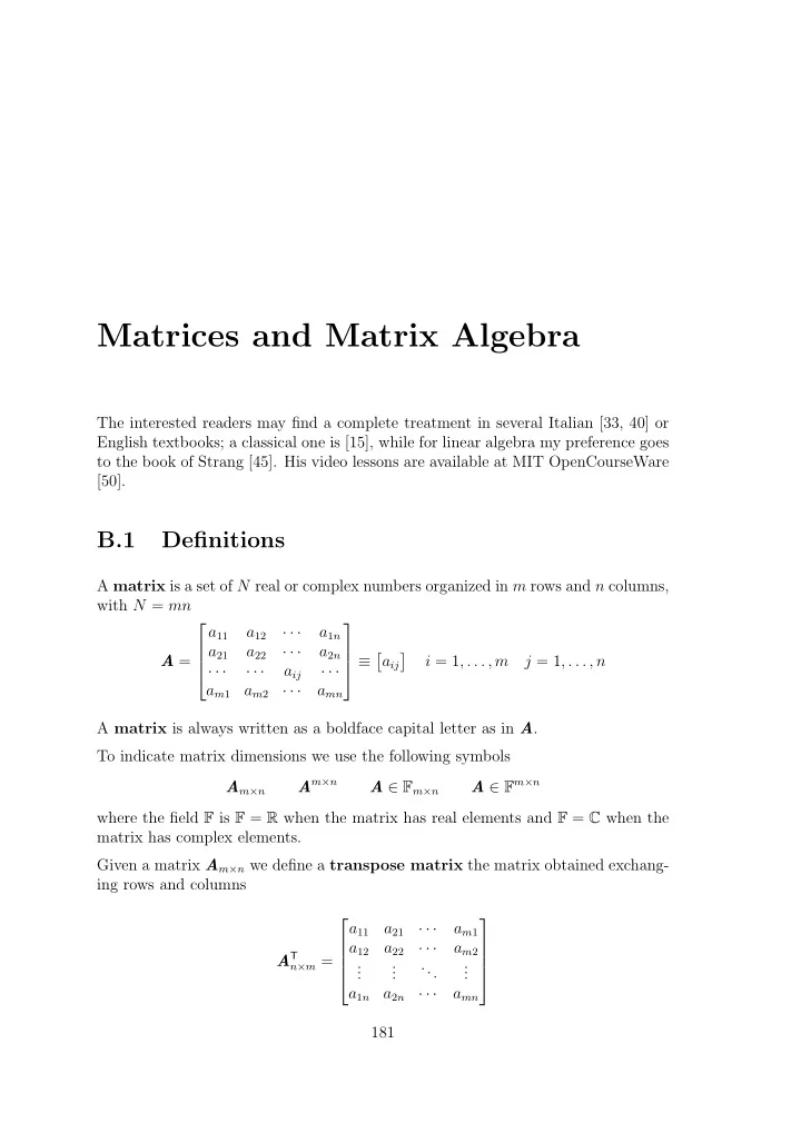
Appendix B Matrices and Matrix Algebra The interested readers may find a complete treatment in several Italian [33, 40] or English textbooks; a classical one is [15], while for linear algebra my preference goes to the book of Strang [45]. His video lessons are available at MIT OpenCourseWare [50]. B.1 Definitions A matrix is a set of N real or complex numbers organized in m rows and n columns, with N = mn   a 11 a 12 · · · a 1 n · · · a 21 a 22 a 2 n   [ ] A =  ≡ a ij i = 1 , . . . , m j = 1 , . . . , n   · · · · · · a ij · · ·  a m 1 a m 2 · · · a mn A matrix is always written as a boldface capital letter as in A . To indicate matrix dimensions we use the following symbols A m × n A ∈ F m × n A ∈ F m × n A m × n where the field F is F = R when the matrix has real elements and F = C when the matrix has complex elements. Given a matrix A m × n we define a transpose matrix the matrix obtained exchang- ing rows and columns   · · · a 11 a 21 a m 1 a 12 a 22 · · · a m 2   A T   n × m = . . . ...  . . .  . . .   a 1 n a 2 n · · · a mn 181

182 Basilio Bona - Dynamic Modelling The following property holds ( A T ) T = A . A matrix is said to be square when m = n A square n × n matrix is upper triangular when a ij = 0 , ∀ i > j   a 11 a 12 · · · a 1 n 0 a 22 · · · a 2 n     A n × n = . . . ...  . . .  . . .   · · · 0 0 a nn A square matrix is lower triangular if its transpose is upper triangular and vicev- ersa.   a 11 0 · · · 0 a 12 a 22 · · · 0   A T   n × n = . . . ...  . . .  . . .   a 1 n a 2 n · · · a nn A real square matrix is said to be symmetric if A − A T = O A = A T → In a real symmetric matrix there are at most n ( n + 1) independent elements. 2 If a matrix K has complex elements k ij = a ij + j b ij (where j = √− 1) its conjugate is K with elements k ij = a ij − j b ij . Given a complex matrix K , an adjoint matrix K ∗ is defined, as the conjugate T = K T transpose K ∗ = K A complex matrix is called self-adjoint or hermitian when K = K ∗ . Some textbooks indicate this matrix as K † or K H . A square matrix is diagonal if a ij = 0 for i ̸ = j   a 1 0 · · · 0 · · · 0 a 2 0     A n × n = diag( a i ) = . . . ...  . . .  . . .   0 0 · · · a n A diagonal matrix is always symmetric and has at most n non zero elements. A square matrix is skew-symmetric or antisymmetric if A + A T = 0 A = − A T → Antisymmetric matrix properties will be described in Appendix B.6.

183 Basilio Bona - Dynamic Modelling B.1.1 Block matrix It is possible to represent a matrix with blocks as   · · · A 11 A 1 n . .  . .  A = . A ij .   · · · A m 1 A mn where the blocks A ij have suitable dimensions. Given the following matrices       · · · A 11 A 1 n A 11 O O A 11 O O . .  .   .  A 1 =  A 2 =  A 3 = O A ij O O A ij . . A ij O     O O A mn · · · O O A mn A m 1 A mn A 1 is upper block triangular , A 2 is lower block triangular , and A 3 is block diagonal � Example B.1.1 Given two matrices A and B   [ 0 − 1 3 ] − 5 4  ; − 2 A = 7 B =  − 3 1 6 4 − 5 Matrix A is 3 × 2, while B is 2 × 3. The transpose matrices are   0 − 3 [ − 1 ] 7 4 A T = B T = − 5 ; 1   − 2 − 5 3 4 6 The matrix   − 4 6 3 − 5 C = 9 2   7 − 1 8 is square and its transpose is   − 4 9 7 C T = 6 2 − 1   − 5 3 8 The matrix   1 2 − 3 D = 2 4 5   − 3 − 6 5

184 Basilio Bona - Dynamic Modelling is symmetrical, since       − 3 − 3 1 2 1 2 0 0 0 D − D T =  −  = 2 4 5 2 4 5 0 0 0     − 3 − 6 − 3 − 6 5 5 0 0 0 The matrix   1 0 0 E = 0 2 0   0 0 3 is diagonal and symmetrical. The matrix   − 4 0 1 F = − 1 0 6   − 6 4 0 is skew-symmetric, since       0 1 − 4 0 − 1 4 0 0 0 F + F T =  +  = − 1 0 6 1 0 − 6 0 0 0     4 − 6 0 − 4 6 0 0 0 0 The 4 × 4 matrix   1 2 3 4 5 6 7 8   G =   9 0 1 2   3 4 5 6 can be written as the following block matrix [ G 11 G 12 ] G = G 21 G 22 with [ 1 ] [ 3 ] 2 4 G 11 = G 21 = 5 6 7 8 [ 9 ] [ 1 ] 0 2 G 12 = G 22 = 3 4 5 6 or     1 2 3 4 G 11 = 5 6 7 G 21 = 8     9 0 1 2 [ ] [ ] G 12 = 3 4 5 G 22 = 6 �

185 Basilio Bona - Dynamic Modelling B.1.2 Matrix algebra Matrices are elements of an algebra , i.e., a vector space together with a product operator . The main operations associated to the matrix algebra are: product by a scalar , sum , and matrix product . Product by a scalar     a 11 a 12 · · · a 1 n αa 11 αa 12 · · · αa 1 n · · · · · · a 21 a 22 a 2 n αa 21 αa 22 αa 2 n         α A = α  = . . . . . . ... ...  . . .   . . .  . . . . . .    a m 1 a m 2 · · · a mn αa m 1 αa m 2 · · · αa mn Sum   · · · a 11 + b 11 a 12 + b 12 a 1 n + b 1 n a 21 + b 21 a 22 + b 22 · · · a 2 n + b 2 n     A + B = . . . ...  . . .  . . .   a m 1 + b m 1 a m 2 + b m 2 · · · a mn + b mn The matrix sum properties are: A + O = existence of a null element A A + B = B + A commutativity ( A + B ) + C = A + ( B + C ) distributivity A T + B T ( A + B ) T = The null (neutral, zero) element O takes the name of null matrix . The subtraction (difference) operation is defined using the scalar α = − 1: A − B = A + ( − 1) B � Example B.1.2 Given the two square matrices A e B     − 1 3 5 0 − 5 4  ; A = 7 − 2 8 B = − 3 1 6    − 2 − 2 1 3 9 5

186 Basilio Bona - Dynamic Modelling and the two scalars α = − 2; β = 5 Matrix C , obtained as a linear combination C = α A + β B is       − 1 − 5 − 31 3 5 0 4 2 10  + 5  = C = − 2 7 − 2 8 − 3 1 6 − 29 9 14     1 3 − 2 9 − 2 5 43 − 16 29 � Matrix product The operation is performed using the well-known rule “ rows by columns ”: the generic element c ij of the matrix product C m × p = A m × n · B n × p is n ∑ c ij = a ik b kj k =1 The bi-linearity of the matrix product is guaranteed, since it is immediate to verify that, given a generic scalar α , the following identity holds: α ( A · B ) = ( α A ) · B = A · ( α B ) The properties of the matrix product are: A · B · C = ( A · B ) · C = A · ( B · C ) A · ( B + C ) = A · B + A · C ( A + B ) · C = A · C + B · C ( A · B ) T = B T · A T In general it is important to notice that • the matrix product is non-commutative: A · B ̸ = B · A , apart from particular cases; • A · B = A · C does not imply B = C , apart from particular cases; • A · B = O does not imply A = O or B = O , apart from particular cases. It is a common habit to omit the · sign of product, so that A · B ≡ AB

187 Basilio Bona - Dynamic Modelling The product between block matrices follows the general rules; for instance given [ A 11 ] [ B 11 ] A 12 B 12 A = B = A 21 A 22 B 21 B 22 The product AB yields [ A 11 B 11 + A 12 B 21 ] A 11 B 12 + A 12 B 22 AB = A 21 B 11 + A 22 B 21 A 21 B 12 + A 22 B 22 � Example B.1.3 Given the two matrices A e B     − 1 3 5 0 − 5 4  ; A = 7 − 2 8 B = − 3 1 6    1 3 − 2 9 − 2 5 We compute C 1 = AB and C 2 = BA as:     36 − 2 39 − 31 22 − 48 − 53 − 19 C 1 = AB = 78 56 C 2 = BA = 16 7     − 27 2 12 − 18 46 19 Now we compute B T A T and see that it is equal to C T 1 :   36 78 − 27 B T A T =  = C T − 2 − 53 2  1 39 56 12 We present a case where AB = AC does not imply B = C . Given       1 0 0 1 0 0 1 0 0 0 1 − 1 0 2 2 0 1 0 A = B = C =       0 − 2 2 0 1 3 0 0 1 We compute the product obtaining   1 0 0 AC = AB = 0 1 − 1   − 2 0 2 We present a case where AB = O does not imply A = O or B = O .     1 0 0 0 0 0  ̸ = O  ̸ = O A = 0 1 − 1 B = 0 1 2   − 2 0 2 0 1 2 AB = O �

188 Basilio Bona - Dynamic Modelling B.1.3 Special matrices Some matrices have special structures Identity matrix A neutral element with respect to the product exists and is called identity matrix . It is a square n × n matrix written is a I n or simply I when no ambiguity arises   1 0 · · · 0 0 1 · · · 0     I = . . . ...  . . .  . . .   · · · 0 0 1 Given a rectangular matrix A m × n the following identities hold A m × n = I m A m × n = A m × n I n Idempotent matrix Given a square matrix A ∈ R n × n , its k -th power is k ∏ A k = A ℓ =1 A matrix is said to be idempotent if A 2 = A A n = A ⇒ � Example B.1.4 Given the A matrix   − 1 3 5 A = 7 − 2 4   − 2 1 3 we compute the power A 3 :   12 60 165 A 3 = AAA = 295 − 68 25   − 60 135 12