App. A: Sequences and difference equations (Part 1, 29 sept) Joakim - PowerPoint PPT Presentation

App. A: Sequences and difference equations (Part 1, 29 sept) Joakim Sundnes 1 , 2 Hans Petter Langtangen 1 , 2 Simula Research Laboratory 1 University of Oslo, Dept. of Informatics 2 Sep 27, 2017

Plan for week 39 Wednesday 27 september Live programming of ex 5.13, 5.29, 5.39 Animations in matplotlib Making our own modules (from Chapter 4) Friday 29 september Live programming of ex 5.39, A.1 Programming of difference equations (Appendix A) Intro to programming of sequences A difference equation for growth and interest A system of (two) difference equations Fibonacci numbers

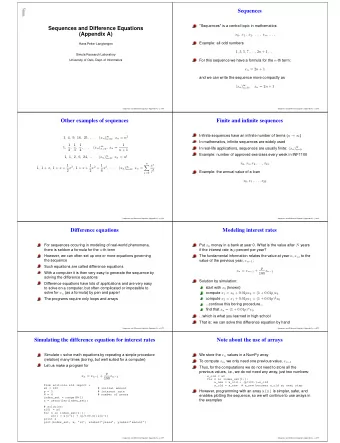
Sequences Sequences is a central topic in mathematics: x 0 , x 1 , x 2 , . . . , x n , . . . , Example: all odd numbers 1 , 3 , 5 , 7 , . . . , 2 n + 1 , . . . For this sequence we have a formula for the n -th term: x n = 2 n + 1 and we can write the sequence more compactly as ( x n ) ∞ n = 0 , x n = 2 n + 1

Other examples of sequences n = 0 , x n = n 2 1 , 4 , 9 , 16 , 25 , . . . ( x n ) ∞ 1 , 1 2 , 1 3 , 1 1 4 , . . . ( x n ) ∞ n = 0 , x n = n + 1 1 , 1 , 2 , 6 , 24 , . . . ( x n ) ∞ n = 0 , x n = n ! n x j 1 , 1 + x , 1 + x + 1 2 x 2 , 1 + x + 1 2 x 2 + 1 6 x 3 , . . . � ( x n ) ∞ n = 0 , x n = j ! j = 0

Finite and infinite sequences Infinite sequences have an infinite number of terms ( n → ∞ ) In mathematics, infinite sequences are widely used In real-life applications, sequences are usually finite: ( x n ) N n = 0 Example: number of approved exercises every week in IN1900 x 0 , x 1 , x 2 , . . . , x 15 Example: the annual value of a loan x 0 , x 1 , . . . , x 20

Difference equations For sequences occuring in modeling of real-world phenomena, there is seldom a formula for the n -th term However, we can often set up one or more equations governing the sequence Such equations are called difference equations With a computer it is then very easy to generate the sequence by solving the difference equations Difference equations have lots of applications and are very easy to solve on a computer, but often complicated or impossible to solve for x n (as a formula) by pen and paper! The programs require only loops and arrays

Modeling interest rates Problem: Put x 0 money in a bank at year 0. What is the value after N years if the interest rate is p percent per year? Solution: The fundamental information relates the value at year n , x n , to the value of the previous year, x n − 1 : p x n = x n − 1 + 100 x n − 1 How to solve for x n ? Start with x 0 , compute x 1 , x 2 , ...

Modeling interest rates Problem: Put x 0 money in a bank at year 0. What is the value after N years if the interest rate is p percent per year? Solution: The fundamental information relates the value at year n , x n , to the value of the previous year, x n − 1 : p x n = x n − 1 + 100 x n − 1 How to solve for x n ? Start with x 0 , compute x 1 , x 2 , ...

Modeling interest rates Problem: Put x 0 money in a bank at year 0. What is the value after N years if the interest rate is p percent per year? Solution: The fundamental information relates the value at year n , x n , to the value of the previous year, x n − 1 : p x n = x n − 1 + 100 x n − 1 How to solve for x n ? Start with x 0 , compute x 1 , x 2 , ...

Solve difference equation for interest rates We solve the equation by repeating a simple procedure (relation) many times (boring, but well suited for a computer!) Program for x n = x n − 1 + ( p / 100 ) x n − 1 : from numpy import * from matplotlib.pyplot import * x0 = 100 # initial amount p = 5 # interest rate N = 4 # number of years index_set = range(N+1) x = zeros(len(index_set)) # Solution: x[0] = x0 for n in index_set[1:]: x[n] = x[n-1] + (p/100.0)*x[n-1] print(x) plot(index_set, x, 'ro') xlabel('years') ylabel('amount') show()

We do not need to store the entire sequence, but it is convenient for programming and later plotting Previous program stores all the x n values in a NumPy array To compute x n , we only need one previous value, x n − 1 Thus, we could only store the two last values in memory: x_old = x0 for n in index_set[1:]: x_new = x_old + (p/100.)*x_old x_old = x_new # x_new becomes x_old at next step However, programming with an array x[n] is simpler, safer, and enables plotting the sequence, so we will continue to use arrays in the examples

Daily interest rate A more relevant model is to add the interest every day The interest rate per day is r = p / D if p is the annual interest rate and D is the number of days in a year A common model in business applies D = 360, but n counts exact (all) days Just a minor change in the model: r x n = x n − 1 + 100 x n − 1 How can we find the number of days between two dates? >>> import datetime >>> date1 = datetime.date(2017, 9, 29) # Sep 29, 2017 >>> date2 = datetime.date(2018, 8, 4) # Aug 4, 2018 >>> diff = date2 - date1 >>> print diff.days 309

Program for daily interest rate from numpy import * from matplotlib.pyplot import * x0 = 100 # initial amount p = 5 # annual interest rate r = p/360.0 # daily interest rate import datetime date1 = datetime.date(2017, 9, 29) date2 = datetime.date(2018, 8, 4) diff = date2 - date1 N = diff.days index_set = range(N+1) x = zeros(len(index_set)) x[0] = x0 for n in index_set[1:]: x[n] = x[n-1] + (r/100.0)*x[n-1] plot(index_set, x, 'ro') xlabel('days') ylabel('amount') show()

But the annual interest rate may change quite often... Varying p means p n : Could not be handled in school (cannot apply p 100 ) n ) x n = x 0 ( 1 + A varying p causes no problems in the program: just fill an array p with correct interest rate for day n Modified program: p = zeros(len(index_set)) # fill p[n] for n in index_set (might be non-trivial...) r = p/360.0 # daily interest rate x = zeros(len(index_set)) x[0] = x0 for n in index_set[1:]: x[n] = x[n-1] + (r[n-1]/100.0)*x[n-1]

Payback of a loan A loan L is paid back with a fixed amount L / N every month over N months + the interest rate of the loan p : annual interest rate, p / 12 : monthly rate Let x n be the value of the loan at the end of month n The fundamental relation from one month to the text: p 12 · 100 x n − 1 + L p x n = x n − 1 + 12 · 100 x n − 1 − ( N ) which simplifies to x n = x n − 1 − L N ( L / N makes the equation nonhomogeneous )

How to make a living from a fortune with constant consumption We have a fortune F invested with an annual interest rate of p percent Every year we plan to consume an amount c n ( n counts years) Let x n be our fortune at year n A fundamental relation from one year to the other is p x n = x n − 1 + 100 x n − 1 − c n Simplest possibility: keep c n constant, but inflation demands c n to increase...

How to make a living from a fortune with inflation-adjusted consumption Assume I percent inflation per year Start with c 0 as q percent of the interest the first year c n then develops as money with interest rate I x n develops with rate p but with a loss c n every year: x n = x n − 1 + p x 0 = F , c 0 = pq 100 x n − 1 − c n − 1 , 10 4 F I c n = c n − 1 + 100 c n − 1 This is a coupled system of two difference equations, but the programming is still simple: we update two arrays, first x[n] , then c[n] , inside the loop (good exercise!)

The mathematics of Fibonacci numbers No programming or math course is complete without an example on Fibonacci numbers: x n = x n − 1 + x n − 2 , x 0 = 1 , x 1 = 1 Mathematical classification This is a homogeneous difference equation of second order (second order means three levels: n , n − 1, n − 2). This classification is important for mathematical solution technique, but not for simulation in a program. Fibonacci derived the sequence by modeling rat populations, but the sequence of numbers has a range of peculiar mathematical properties and has therefore attracted much attention from mathematicians.

Program for generating Fibonacci numbers import sys from numpy import zeros N = int(sys.argv[1]) x = zeros(N+1, int) x[0] = 1 x[1] = 1 for n in range(2, N+1): x[n] = x[n-1] + x[n-2] print(n, x[n])

Fibonacci numbers can cause overflow in NumPy arrays Run the program with N = 100: 2 2 3 3 4 5 5 8 6 13 ... 91 7540113804746346429 fibonacci.py:9: RuntimeWarning: overflow encountered in long_scalars x[n] = x[n-1] + x[n-2] 92 -6246583658587674878 Note: NumPy ’int’ supports up to 9223372036854775807 Can be fixed by avoiding arrays, and changing from NumPy int to standard Python int See the book for details

Summary of difference equations (part 1) A sequence where x n is expressed by x n − 1 , x n − 2 etc is a difference equation In general no explicit formula for x n , so hard to solve on paper for large n Easy to solve in Python: Start with x 0 Compute x n from x n − 1 i a for loop Easily extended to systems of difference equations Just update all the sequences in the same for loop