An Average-Case Analysis for Rate-Monotonic Multiprocessor - PowerPoint PPT Presentation

An Average-Case Analysis for Rate-Monotonic Multiprocessor Real-time Scheduling Andreas Karrenbauer & Thomas Rothvoß Institute of Mathematics EPFL, Lausanne ESA 2009

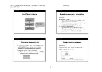
Real-time Scheduling Given: synchronous tasks τ 1 , . . . , τ n where task τ i ◮ is periodic with period p ( τ i ) ◮ has running time c ( τ i ) ◮ has implicit deadline W.l.o.g.: Task τ i releases job of length c ( τ i ) at 0 , p ( τ i ) , 2 p ( τ i ) , . . . Scheduling policy: ◮ multiprocessor ◮ fixed priority ◮ pre-emptive

b b b Example c ( τ 1 ) = 1 p ( τ 1 ) = 2 time 0 1 2 3 4 5 6 7 8 9 10 c ( τ 2 ) = 2 p ( τ 2 ) = 5

b b b Example Theorem (Liu & Layland ’73) 1 Optimal priorities: p ( τ i ) for τ i (Rate-monotonic Schedule) c ( τ 1 ) = 1 p ( τ 1 ) = 2 time 0 1 2 3 4 5 6 7 8 9 10 c ( τ 2 ) = 2 p ( τ 2 ) = 5

b b b Example Theorem (Liu & Layland ’73) 1 Optimal priorities: p ( τ i ) for τ i (Rate-monotonic Schedule) c ( τ 1 ) = 1 p ( τ 1 ) = 2 time 0 1 2 3 4 5 6 7 8 9 10 c ( τ 2 ) = 2 p ( τ 2 ) = 5

b b b Example Theorem (Liu & Layland ’73) 1 Optimal priorities: p ( τ i ) for τ i (Rate-monotonic Schedule) c ( τ 1 ) = 1 p ( τ 1 ) = 2 time 0 1 2 3 4 5 6 7 8 9 10 c ( τ 2 ) = 2 p ( τ 2 ) = 5

b b b Example Theorem (Liu & Layland ’73) 1 Optimal priorities: p ( τ i ) for τ i (Rate-monotonic Schedule) c ( τ 1 ) = 1 p ( τ 1 ) = 2 time 0 1 2 3 4 5 6 7 8 9 10 c ( τ 2 ) = 2 p ( τ 2 ) = 5 Definition u ( τ ) = c ( τ ) p ( τ ) = utilization of task τ

Feasibility test Theorem (Lehoczky et al. ’89) If p ( τ 1 ) ≤ . . . ≤ p ( τ n ) then the response time r ( τ i ) in a RM-schedule is the smallest value s.t. � r ( τ i ) � � c ( τ i ) + c ( τ j ) ≤ r ( τ i ) p ( τ j ) j<i 1 machine suffices ⇔ ∀ i : r ( τ i ) ≤ p ( τ i ) .

Feasibility test Theorem (Lehoczky et al. ’89) If p ( τ 1 ) ≤ . . . ≤ p ( τ n ) then the response time r ( τ i ) in a RM-schedule is the smallest value s.t. � r ( τ i ) � � c ( τ i ) + c ( τ j ) ≤ r ( τ i ) p ( τ j ) j<i 1 machine suffices ⇔ ∀ i : r ( τ i ) ≤ p ( τ i ) . Theorem (Eisenbrand & R. ’08) Computing a response time r ( τ i ) is NP -hard.

Feasibility test Theorem (Lehoczky et al. ’89) If p ( τ 1 ) ≤ . . . ≤ p ( τ n ) then the response time r ( τ i ) in a RM-schedule is the smallest value s.t. � r ( τ i ) � � c ( τ i ) + c ( τ j ) ≤ r ( τ i ) p ( τ j ) j<i 1 machine suffices ⇔ ∀ i : r ( τ i ) ≤ p ( τ i ) . Theorem (Eisenbrand & R. ’08) Computing a response time r ( τ i ) is NP -hard. Theorem (Liu & Layland ’73) u ( S ) = � τ ∈S u ( τ ) ≤ ln(2) ≈ 69% ⇒ 1 machine suffices

Feasibility test Theorem (Lehoczky et al. ’89) If p ( τ 1 ) ≤ . . . ≤ p ( τ n ) then the response time r ( τ i ) in a RM-schedule is the smallest value s.t. � r ( τ i ) � � c ( τ i ) + c ( τ j ) ≤ r ( τ i ) p ( τ j ) j<i 1 machine suffices ⇔ ∀ i : r ( τ i ) ≤ p ( τ i ) . Theorem (Eisenbrand & R. ’08) Computing a response time r ( τ i ) is NP -hard. Theorem (Liu & Layland ’73) u ( S ) = � τ ∈S u ( τ ) ≤ ln(2) ≈ 69% ⇒ 1 machine suffices Observation If p ( τ 1 ) | p ( τ 2 ) | . . . | p ( τ n ): 1 machine suffices ⇔ u ( S ) ≤ 1

Feasibility test (2) Lemma (Burchard et al. ’95) For tasks S = { τ 1 , . . . , τ n } define

Feasibility test (2) Lemma (Burchard et al. ’95) For tasks S = { τ 1 , . . . , τ n } define α ( τ i ) := log 2 p ( τ i ) − ⌊ log 2 p ( τ i ) ⌋

Feasibility test (2) Lemma (Burchard et al. ’95) For tasks S = { τ 1 , . . . , τ n } define α ( τ i ) := log 2 p ( τ i ) − ⌊ log 2 p ( τ i ) ⌋ 1 2 4 8 periods

Feasibility test (2) Lemma (Burchard et al. ’95) For tasks S = { τ 1 , . . . , τ n } define α ( τ i ) := log 2 p ( τ i ) − ⌊ log 2 p ( τ i ) ⌋ p ( τ 1 ) p ( τ 2 ) p ( τ 3 ) 1 2 4 8 periods

Feasibility test (2) Lemma (Burchard et al. ’95) For tasks S = { τ 1 , . . . , τ n } define α ( τ i ) := log 2 p ( τ i ) − ⌊ log 2 p ( τ i ) ⌋ p ( τ 1 ) p ( τ 2 ) p ( τ 3 ) 1 2 4 8 periods 0 1

Feasibility test (2) Lemma (Burchard et al. ’95) For tasks S = { τ 1 , . . . , τ n } define α ( τ i ) := log 2 p ( τ i ) − ⌊ log 2 p ( τ i ) ⌋ p ( τ 1 ) p ( τ 2 ) p ( τ 3 ) 1 2 4 8 periods α ( τ 1 ) 0 1

Feasibility test (2) Lemma (Burchard et al. ’95) For tasks S = { τ 1 , . . . , τ n } define α ( τ i ) := log 2 p ( τ i ) − ⌊ log 2 p ( τ i ) ⌋ p ( τ 1 ) p ( τ 2 ) p ( τ 3 ) 1 2 4 8 periods α ( τ 2 ) α ( τ 1 ) 0 1

Feasibility test (2) Lemma (Burchard et al. ’95) For tasks S = { τ 1 , . . . , τ n } define α ( τ i ) := log 2 p ( τ i ) − ⌊ log 2 p ( τ i ) ⌋ p ( τ 1 ) p ( τ 2 ) p ( τ 3 ) 1 2 4 8 periods α ( τ 2 ) α ( τ 1 ) α ( τ 3 ) 0 1

Feasibility test (2) Lemma (Burchard et al. ’95) For tasks S = { τ 1 , . . . , τ n } define α ( τ i ) := log 2 p ( τ i ) − ⌊ log 2 p ( τ i ) ⌋ and β ( S ) := max i,j | α ( τ i ) − α ( τ j ) | p ( τ 1 ) p ( τ 2 ) p ( τ 3 ) 1 2 4 8 periods α ( τ 2 ) α ( τ 1 ) α ( τ 3 ) 0 1 β

Feasibility test (2) Lemma (Burchard et al. ’95) For tasks S = { τ 1 , . . . , τ n } define α ( τ i ) := log 2 p ( τ i ) − ⌊ log 2 p ( τ i ) ⌋ and β ( S ) := max i,j | α ( τ i ) − α ( τ j ) | One machine suffices if u ( S ) ≤ 1 − β ( S ) . p ( τ 1 ) p ( τ 2 ) p ( τ 3 ) 1 2 4 8 periods α ( τ 2 ) α ( τ 1 ) α ( τ 3 ) 0 1 β

Algorithms for Multiprocessor Scheduling

Algorithms for Multiprocessor Scheduling Known results: ◮ NP -hard (generalization of Bin Packing)

Algorithms for Multiprocessor Scheduling Known results: ◮ NP -hard (generalization of Bin Packing) ◮ asymp. 1.75-apx [Burchard et al. ’95]

Algorithms for Multiprocessor Scheduling Known results: ◮ NP -hard (generalization of Bin Packing) ◮ asymp. 1.75-apx [Burchard et al. ’95] ◮ asymp. (1 + ε )-apx (with resource augmentation) in O ε (1) · n (1 /ε ) O (1) [Eisenbrand & R. ’08]

Algorithms for Multiprocessor Scheduling Known results: ◮ NP -hard (generalization of Bin Packing) ◮ asymp. 1.75-apx [Burchard et al. ’95] ◮ asymp. (1 + ε )-apx (with resource augmentation) in O ε (1) · n (1 /ε ) O (1) [Eisenbrand & R. ’08] Some papers: 1. Sort tasks w.r.t. some criteria (e.g. p ( τ i ) , u ( τ i ) , α ( τ i ))

Algorithms for Multiprocessor Scheduling Known results: ◮ NP -hard (generalization of Bin Packing) ◮ asymp. 1.75-apx [Burchard et al. ’95] ◮ asymp. (1 + ε )-apx (with resource augmentation) in O ε (1) · n (1 /ε ) O (1) [Eisenbrand & R. ’08] Some papers: 1. Sort tasks w.r.t. some criteria (e.g. p ( τ i ) , u ( τ i ) , α ( τ i )) 2. Distribute tasks in a First Fit/Next Fit way using a sufficient feasibility criterion

Algorithms for Multiprocessor Scheduling Known results: ◮ NP -hard (generalization of Bin Packing) ◮ asymp. 1.75-apx [Burchard et al. ’95] ◮ asymp. (1 + ε )-apx (with resource augmentation) in O ε (1) · n (1 /ε ) O (1) [Eisenbrand & R. ’08] Some papers: 1. Sort tasks w.r.t. some criteria (e.g. p ( τ i ) , u ( τ i ) , α ( τ i )) 2. Distribute tasks in a First Fit/Next Fit way using a sufficient feasibility criterion 3. Perform experiments with randomly chosen tasks

Algorithms for Multiprocessor Scheduling Known results: ◮ NP -hard (generalization of Bin Packing) ◮ asymp. 1.75-apx [Burchard et al. ’95] ◮ asymp. (1 + ε )-apx (with resource augmentation) in O ε (1) · n (1 /ε ) O (1) [Eisenbrand & R. ’08] Some papers: 1. Sort tasks w.r.t. some criteria (e.g. p ( τ i ) , u ( τ i ) , α ( τ i )) 2. Distribute tasks in a First Fit/Next Fit way using a sufficient feasibility criterion 3. Perform experiments with randomly chosen tasks Definition Probability distribution: ◮ Adversary gives p ( τ i ) ◮ u ( τ i ) ∈ [0 , 1] uniformly at random

Waste Definition Waste of a solution: #machines − u ( S ).

Waste Definition Waste of a solution: #machines − u ( S ). 1 0 M1 M2 M3

Waste Definition Waste of a solution: #machines − u ( S ). 1 τ 0 M1 M2 M3

Waste Definition Waste of a solution: #machines − u ( S ). 1 τ u ( τ ) 0 M1 M2 M3

Waste Definition Waste of a solution: #machines − u ( S ). waste 1 τ u ( τ ) 0 M1 M2 M3

Our algorithm First Fit Matching Periods (FFMP): 1. Sort: 0 ≤ α ( τ 1 ) ≤ α ( τ 2 ) ≤ . . . ≤ α ( τ n ) < 1 2. First Fit: FOR i = 1 , . . . , n DO ◮ Assign τ i to first machine P with u ( P + τ i ) ≤ 1 − β ( P + τ i )

Our algorithm First Fit Matching Periods (FFMP): 1. Sort: 0 ≤ α ( τ 1 ) ≤ α ( τ 2 ) ≤ . . . ≤ α ( τ n ) < 1 2. First Fit: FOR i = 1 , . . . , n DO ◮ Assign τ i to first machine P with u ( P + τ i ) ≤ 1 − β ( P + τ i ) M1 M2 M3 u ( τ ) input α ≈ 1 α ≈ 0

Our algorithm First Fit Matching Periods (FFMP): 1. Sort: 0 ≤ α ( τ 1 ) ≤ α ( τ 2 ) ≤ . . . ≤ α ( τ n ) < 1 2. First Fit: FOR i = 1 , . . . , n DO ◮ Assign τ i to first machine P with u ( P + τ i ) ≤ 1 − β ( P + τ i ) M1 M2 M3 u ( τ ) input