Amortized Analysis Pedro Ribeiro DCC/FCUP 2018/2019 Pedro Ribeiro - PowerPoint PPT Presentation
Amortized Analysis Pedro Ribeiro DCC/FCUP 2018/2019 Pedro Ribeiro (DCC/FCUP) Amortized Analysis 2018/2019 1 / 30 Amortized Analysis In amortized analysis we are concerned about the average over a sequence of operations Some operations
Amortized Analysis Pedro Ribeiro DCC/FCUP 2018/2019 Pedro Ribeiro (DCC/FCUP) Amortized Analysis 2018/2019 1 / 30
Amortized Analysis In amortized analysis we are concerned about the average over a sequence of operations ◮ Some operations may be costly, but others may be quicker, and in the end they even out ◮ Typically applied to the analysis of a data structure This is different from the regular worst case analysis , where the worst cost of one operation is analyzed ◮ There might be correlations between operations and worst case per operation might be too pessimistic because the only way of having an expensive operation might be to have a lot of cheap ones before This is different from average case analysis , and there is no probability or expectation involved ◮ Amortized analysis still gives us a view of the worst possible scenario Pedro Ribeiro (DCC/FCUP) Amortized Analysis 2018/2019 2 / 30
Amortized Analysis Definitions Amortized cost The amortized cost per operation for a sequence of n operations is the total cost of the operations divided by n Amortized complexity The amortized sequence complexity is the worst case sequence complexity (that is, the maximum possible total cost over all possible sequences of n operations) divided by n Pedro Ribeiro (DCC/FCUP) Amortized Analysis 2018/2019 3 / 30
Methods for Amortized Analysis Aggregate method ( total cost ) Examine total cost of operations and see the average Accounting method ( banker’s view ) Impose extra charge on inexpensive operations, saving for future expensive operations Potential method ( physicist’s view ) Define a (non-negative) potential function on the data structure state and use it to bound the cost Pedro Ribeiro (DCC/FCUP) Amortized Analysis 2018/2019 4 / 30
Intuition and Motivation Real Life intuition: consider the monthly cost of living, a sequence of 12 operations: Pedro Ribeiro (DCC/FCUP) Amortized Analysis 2018/2019 5 / 30
Aggregate Method What is the amortized cost per month (operation)? Just sum up the cost of all months (operations) and divide by the number of months (operations) Aggregate method: sum of all months is 5,400€, which divided by 12 months gives an amortized cost of 450€ per month. Pedro Ribeiro (DCC/FCUP) Amortized Analysis 2018/2019 6 / 30
Accounting method Instead of computing the average after knowing the total cost, we may think of it from a different angle: How much money do I need to earn each month in order to keep living , never being broke and always be able to pay the bills? Accounting method: If I always earn 450€, then I will always have enough money to pay the bill and never become broke: ◮ When I earn more than expenditures, I save some money for the future ◮ When I earn less than expenditures, I use the money I saved Pedro Ribeiro (DCC/FCUP) Amortized Analysis 2018/2019 7 / 30
A first example: stack as an array Let’s have a look at a data structure example. Imagine I have a stack implemented as an array supporting the following operations: push( x ) - add an element x to the top of the stack x = pop() - remove and return the element on the top What happens when I need to push an element and the array is full ? We need to create a new, bigger array, copy the existing elements, and continue from there This is an expensive operation and a push that does this is going to cost a lot Pedro Ribeiro (DCC/FCUP) Amortized Analysis 2018/2019 8 / 30
Stack as an array Let’s first establish a cost model: Inserting an element into an existing array costs 1 Removing an element from an array costs 1 Allocating a new array costs 0 (zero) This means a push or pop without resizing costs 1, and a resize would cost n , with n elements being copied to the new array Pedro Ribeiro (DCC/FCUP) Amortized Analysis 2018/2019 9 / 30
Stack as an array What would be a good strategy for resizing the array? A first strategy for resizing Each time the array is full, increment its size by one What is the cost of this strategy? Let’s use the aggregate method starting from an empty array of size 1: i =1 i = ( n +1) n = O ( n 2 ) Total cost of n pushes = 1 + 2 + . . . + n = � n 2 The average over n operations, our amortized cost , is O ( n ). Can we do better ? (than amortized linear cost) Pedro Ribeiro (DCC/FCUP) Amortized Analysis 2018/2019 10 / 30
Stack as an array Let’s try something different: A better strategy for resizing Each time the array is full, double its size Cost? Let’s use the aggregate method as before: The cost of insertions is just n The cost of resizes is 1 + 2 + 4 + . . . + 2 i for some 2 i < n This sum is smaller than 2 n Total cost of n pushes = cost(insertions) + cost(resizes) < 3 n Average over n operations is < 3, i.e., our amortized cost , is O (1). Pedro Ribeiro (DCC/FCUP) Amortized Analysis 2018/2019 11 / 30
Stack as an array Using amortized analysis we have shown that doubling the size of the array is a good strategy with constant amortized time (per operation) ◮ What would a (non amortized) regular worst case analysis say? ◮ ”Increase size by 100 when full” would not be a good strategy. Why? ◮ What about a strategy for saving (unused) space when popping ? Would halving the array be good? We’ll discuss that on the exercises :) We are (still) missing the other methods ( accounting and potential ). Let’s have a look at how they would work in this example. Pedro Ribeiro (DCC/FCUP) Amortized Analysis 2018/2019 12 / 30
Stack as an array - Accounting method How much money do we need to earn for each push operation, so that all future operations can be paid for? Earn $1 for each push ◮ We spend that $1 for inserting (the ”insert-dollar” ) ◮ When we need to copy this element to a new array (when resizing), we don’t have enough money... BROKE! Earn $2 for each push ◮ $1 for inserting (the ”insert-dollar” ) ◮ $1 for copying to a new array (the ”copy-dollar” ) ◮ When if we need to copy it again for a second time (during a new resize)? ... BROKE! Pedro Ribeiro (DCC/FCUP) Amortized Analysis 2018/2019 13 / 30
Stack as an array - Accounting method Earn $3 for each push ◮ $1 for inserting (the ”insert-dollar” ) ◮ $1 for copying to a new array (the ”copy-dollar” ) ◮ $1 for recharging old elements that have spent their copy-dollars to a new array (the ”recharge-dollar” ) NEVER GO BROKE! We will always have enough new elements sparing enough money for all the old elements because of the way we resize: TWICE the old size Amortized cost of 3 (as before) which is O (1) Pedro Ribeiro (DCC/FCUP) Amortized Analysis 2018/2019 14 / 30
Stack as an array - Potential method The potential method uses an idea similar to the banker’s view but using a different methodology Suppose we can define a potential function Φ (”Phi”) on the state of a data structure with the following properties: Φ( s 0 ) = 0 here s 0 is the initial state of the data structure Φ( s t ) ≥ 0 for all states s t occurring during the sequence of operations Intuitively, the potential function should keep track of the ”precharged cost” at any given time, measuring how much we have ”saved” for future operations, such as in the banker’s method. The difference is that it depends only on the current state of the data structure , regardless of the operations that got us in that state Pedro Ribeiro (DCC/FCUP) Amortized Analysis 2018/2019 15 / 30
Stack as an array - Potential method Armed with this, we can define the amortized cost of an operation as c + Φ ( s ′ ) − Φ ( s ) Where c is the actual cost of the operation and s and s ′ are the states of the data structure before and after the operation, respectively: Amortized cost is the actual cost plus the change in potential Now, consider a sequence of n operations with actual costs c 0 , c 1 , . . . , c n − 1 leading from state s 0 to states s 1 , s 2 , . . . , s n . The total amortized cost is equal to the sums of amortized cost: [ c 0 + Φ( s 1 ) − Φ( s 0 )] + [ c 1 + Φ( s 2 ) − Φ( s 1 )] + . . . + [ c s − 1 + Φ( s n ) − Φ( s n − 1 )] = c 0 + c 1 + . . . + c n − 1 + Φ( s n ) − Φ( s 0 ) = c 0 + c 1 + . . . + c n − 1 + Φ( s n ) Because Φ is always positive, we are overestimating the actual cost by Φ( s n ) and the amortized cost is an upper bound on the actual cost ! Pedro Ribeiro (DCC/FCUP) Amortized Analysis 2018/2019 16 / 30
Stack as an array - Potential method Let’s choose a suitable potential function for our case: Let Φ( s ) be 2x the nr of elements in the array after the midpoint Φ( s ) = max (0 , 2( n − m / 2)) = max (0 , 2 n − m ) where n is the number of elements in the array and m the size of the array. (Note how this corresponds to the surplus money in the banker’s method) Φ( s 0 ) = 0 and Φ( s t ) ≥ 0 for all states s t as required Now we need to show that the amortized cost is O (1) Consider a single push operation: If n < m , then the actual cost is 1 and m does not change. The potential increases by at most 2 (when 2 n > m − 1). So, the amortized cost is at most 1 + 2 = 3. If n == m , then the actual cost is n + 1, but the potential drops from n to 2, which means the amortized cost is n + 1 + (2 − n ) = 3 And we have our constant amortized cost of 3! Pedro Ribeiro (DCC/FCUP) Amortized Analysis 2018/2019 17 / 30
Recommend
More recommend
Explore More Topics
Stay informed with curated content and fresh updates.
