Algoritmi per la Bioinformatica To abstract from specific computers - PDF document

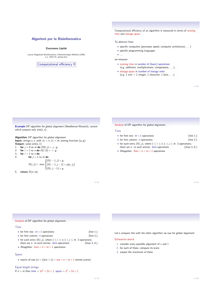
Computational e ffi ciency of an algorithm is measured in terms of running time and storage space. Algoritmi per la Bioinformatica To abstract from • specific computers (processor speed, computer architecture, . . . ) Zsuzsanna Lipt´ ak • specific programming languages • . . . Laurea Magistrale Bioinformatica e Biotechnologie Mediche (LM9) a.a. 2014/15, spring term we measure Computational e ffi ciency II • running time in number of (basic) operations (e.g. additions, multiplications, comparisons, . . . ), • storage space in number of storage units (e.g. 1 unit = 1 integer, 1 character, 1 byte, . . . ). 2 / 23 Analysis of DP algorithm for global alignment: Example DP algorithm for global alignment (Needleman-Wunsch), variant which outputs only sim ( s , t ). Time • for first row: m + 1 operations (line 1.) Algorithm DP algorithm for global alignment • for first column: n operations (line 2.) Input: strings s , t , with | s | = n , | t | = m ; scoring function ( p , g ) • for each entry D ( i , j ), where 1 ≤ i ≤ n , 1 ≤ j ≤ m : 3 operations; Output: value sim ( s , t ) there are n · m such entries: 3 nm operations (lines 3.,4.) 1. for j = 0 to m do D (0 , j ) ← j · g ; 2. for i = 1 to n do D ( i , 0) ← i · g ; • Altogether: 3 nm + n + m + 1 operations 3. for i = 1 to n do 4. for j = 1 to m do 8 D ( i − 1 , j ) + g > < D ( i , j ) ← max D ( i − 1 , j − 1) + p ( s i , t j ) > : D ( i , j − 1) + g 5. return D ( n , m ); 3 / 23 4 / 23 Analysis of DP algorithm for global alignment: Time • for first row: m + 1 operations (line 1.) Let’s compare this with the other algorithm we saw for global alignment: • for first column: n operations (line 2.) Exhaustive search • for each entry D ( i , j ), where 1 ≤ i ≤ n , 1 ≤ j ≤ m : 3 operations; there are n · m such entries: 3 nm operations (lines 3.,4.) 1. consider every possible alignment of s and t • Altogether: 3 nm + n + m + 1 operations 2. for each of these, compute its score 3. output the maximum of these Space • matrix of size ( n + 1)( m + 1) = nm + n + m + 1 entries (units) Equal length strings If n = m then time = 3 n 2 + 2 n + 1, space = n 2 + 2 n + 1 4 / 23 5 / 23

Algorithm Exhaustive search for global alignment Input: strings s , t , with | s | = n , | t | = m ; scoring function ( p , g ) Output: value sim ( s , t ) Analysis of Exhaustive search: 1. int max = ( n + m ) g ; 2. for each alignment A of s and t (in some order) 3. do if score ( A ) > max • Time: next slides 4. then max ← score ( A ); • Space: exercise 5. return max; Note: 1. The variable max is needed for storing the highest score so far seen. 2. The initial value of max is the score of some alignment of s , t (which one?) 6 / 23 7 / 23 Analysis of Exhaustive search (time): Analysis of Exhaustive search (time): • for every alignment (line 2.) • for every alignment (line 2.) no. of al’s • compute its score (line 3.) • compute its score (line 3.) length of al. time = no. of alignments · length of alignment | {z } | {z } N ( n , m ) between max( n , m ) and n + m 8 / 23 8 / 23 Analysis of Exhaustive search (time): So we have, for | s | = | t | = n : • DP algo: 3 n 2 + 2 n + 1 operations • for every alignment (line 2.) no. of al’s • Exhaustive search: at least N ( n , n ) · n operations • compute its score (line 3.) length of al. Let’s compare the two functions for increasing n : time = no. of alignments · length of alignment | {z } | {z } 1 2 3 4 5 10 100 1000 n N ( n , m ) between max( n , m ) and n + m . . . 3 n 2 + 2 n + 1 6 17 34 57 86 321 30 201 3 002 001 . . . ⇡ 80 · 10 6 ⇡ 2 · 10 77 ⇡ 10 700 N ( n , n ) · n 3 26 189 1284 8415 . . . Simplify analysis: Let’s look at two equal length strings | s | = | t | = n : The DP algorithm is much faster than the exhaustive search algorithm, N ( n , n ) · n ≤ time ≤ N ( n , n ) · 2 n because its running time increases much slower as the input size increases. But how much? We have seen: N ( n , n ) > 2 n , so time ≥ 2 n · n . 8 / 23 9 / 23

Algorithm analysis Algorithm analysis • We measure running time and storage space, measured in no. of • We measure running time and storage space, measured in no. of operations and no. of storage units. operations and no. of storage units. • We want to know how our algo performs depending on the size of the input (bigger input = more time/space), i.e. as functions of the input size (usually denoted n , m ). 10 / 23 10 / 23 Algorithm analysis Algorithm analysis • We measure running time and storage space, measured in no. of • We measure running time and storage space, measured in no. of operations and no. of storage units. operations and no. of storage units. • We want to know how our algo performs depending on the size of the • We want to know how our algo performs depending on the size of the input (bigger input = more time/space), i.e. as functions of the input input (bigger input = more time/space), i.e. as functions of the input size (usually denoted n , m ). size (usually denoted n , m ). • We are interested in the algorithm’s behaviour for large inputs. • We are interested in the algorithm’s behaviour for large inputs. • We want to know the growth behaviour, i.e. how time/space requirements change as input increases. 10 / 23 10 / 23 Algorithm analysis Consider 3 algorithms A , B , C : input size n running t. 10 20 What happened when input doubled? • We measure running time and storage space, measured in no. of A n 10 20 operations and no. of storage units. n 2 B 100 400 • We want to know how our algo performs depending on the size of the 2 n C 1024 1 048 576 input (bigger input = more time/space), i.e. as functions of the input size (usually denoted n , m ). • We are interested in the algorithm’s behaviour for large inputs. • We want to know the growth behaviour, i.e. how time/space requirements change as input increases. • We want an upper bound, i.e. on any input how much time/space needed at most? (worst-case analysis) 10 / 23 11 / 23

Consider 3 algorithms A , B , C : Consider 3 algorithms A , B , C : input size n input size n running t. 10 20 What happened when input doubled? running t. 10 20 What happened when input doubled? A 10 20 doubled A 10 20 doubled n n n 2 n 2 B 100 400 quadrupled B 100 400 quadrupled 2 n 2 n C 1024 1 048 576 squared C 1024 1 048 576 squared Now 3 algorithms A 0 , B 0 , C 0 : input size n running t. 10 20 What happened when input doubled? A 0 3 n 30 60 3 n 2 B 0 300 1200 C 0 3 · 2 n 3072 3 145 728 11 / 23 11 / 23 The O -notation allows us to abstract from constants (3 n vs. n ) and other Consider 3 algorithms A , B , C : details which are not important for the growth behaviour of functions. input size n running t. 10 20 What happened when input doubled? Definition (O-classes) A n 10 20 doubled Given a function f : N → R , then O ( f ( n )) is the class (set) of functions n 2 B 100 400 quadrupled g ( n ) s.t.: 2 n C 1024 1 048 576 squared There exists a c > 0 and an n 0 ∈ N s.t. for all n ≥ n 0 : g ( n ) ≤ c · f ( n ). Now 3 algorithms A 0 , B 0 , C 0 : input size n running t. 10 20 What happened when input doubled? A 0 3 n 30 60 doubled 3 n 2 B 0 300 1200 quadrupled 3 · 2 n C 0 3072 3 145 728 1 / 3 of squared 11 / 23 12 / 23 Example The O -notation allows us to abstract from constants (3 n vs. n ) and other 3 n 2 + 2 n + 1 ∈ O ( n 2 ) details which are not important for the growth behaviour of functions. Recall definition Definition (O-classes) g ( n ) ∈ O ( f ( n )) if Given a function f : N → R , then O ( f ( n )) is the class (set) of functions there exists a c > 0 and an n 0 ∈ N s.t. for all n ≥ n 0 : g ( n ) ≤ c · f ( n ). g ( n ) s.t.: Proof There exists a c > 0 and an n 0 ∈ N s.t. for all n ≥ n 0 : g ( n ) ≤ c · f ( n ). We then say that g ( n ) ∈ O ( f ( n )) or g ( n ) = O ( f ( n )) n 1 2 3 4 5 | {z } 3 n 2 + 2 n + 1 Careful, this is not an ”equality”! 6 17 34 57 86 4 n 2 4 16 36 64 100 Meaning: “ g is smaller or equal than f (w.r.t. growth behaviour)” “ g does not grow faster than f ” 12 / 23 13 / 23