AIRS Activities AIRS Activities at NOAA/NESDIS at NOAA/NESDIS - PowerPoint PPT Presentation

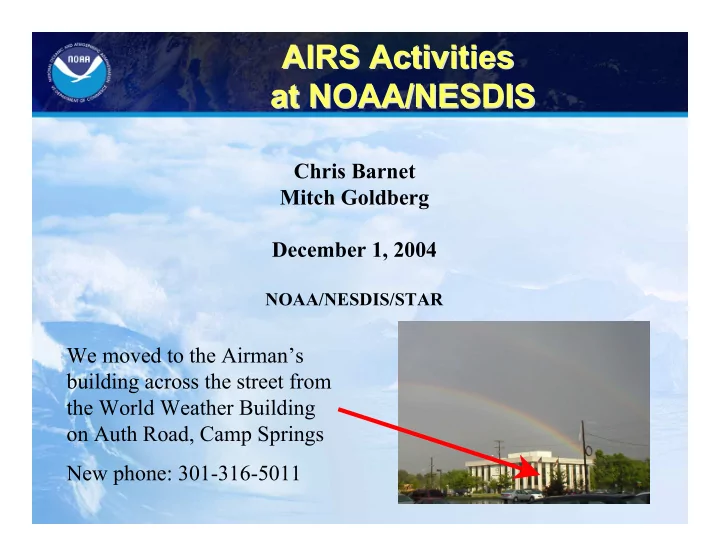
AIRS Activities AIRS Activities at NOAA/NESDIS at NOAA/NESDIS Chris Barnet Mitch Goldberg December 1, 2004 NOAA/NESDIS/STAR We moved to the Airman’s building across the street from the World Weather Building on Auth Road, Camp Springs New phone: 301-316-5011

Topics Covered • Cloud Clearing Risk Reduction Activities – Risk reduction w.r.t. a failure of AMSU – Improving cloud clearing: emissivity cross-talk issues. • Trace Gas Products – Improved first guess states for carbon gases. – Product averaging functions. • L2 issues. – Convergence in water and trace gas retrievals. – Cij • Summary of NOAA/NESDIS AIRS Datasets • Summary of recommendations for v5.0 2

Cloud Clearing Risk Reduction Nick Nalli Walter Wolf Lihang Zhou Collaboration with Mous Chahine, Bob Knuteson, and Dave Tobin 3

Cloud Clearing Risk Reduction Options Currently Being Explored • Operate CC from forecast model (AVN or GDAS) – Concept works (ASTM 3/30/04) – Recommend installation of option for v5, evaluate in frontal situations. • Use a regression trained on cloud contaminated radiances. – Concept works (ASTM 3/30/04) – Minor code changes to allow a 2 nd set of coef’s – Recommend installation of option for v5. • Use MODIS, convolved to AIRS FOV’s – Use MODIS as a QA for AIRS CCR’s (Mitch will discuss this) – MODIS/AIRS CCR regression is under study (Mitch will discuss this) – MODIS/AIRS CCR physical approach is in development. • SW/LW iteration technique (a.k.a. IR cloud clearing). – Preliminary algorithm discussed (3/30/04) Concept needs development. – This approach has many applications for future sounders. – Will begin working out the details in FY05. 4

Cloud Clearing Risk Reduction Emissivity Issues • Emissivity regression retrieval does not seem to be working well – Latest upgrades (4 surface types) is an improvement, but typically produces erroneous spectral structure over land, especially desert, snow, and ice, affecting ozone & water retrievals. – These occur in ≈ 10% of the cases. – We will investigate improving the training & surface type selection. • Emissivity physical retrieval still has major problems. – Recent upgrades rely more on the regression for spectral shape. – It is now clear that Tskin and emissivity are not separated well. • Three experiments are shown to illustrate the issue. 1. “d60” V4.0 emulation (2 _, 1 _) 2. “d61” uses NOAA REG + SVD to solve for 15 _ & 1 _ 3. “d62” Does not NOAA Reg. Assume an emissivity value at one frequency and solves for relative emissivity Land: _(831 cm -1 ) = 0.98 Ocean: _(900 cm -1 ) = Wu/Masuda 5 Snow/Ice: _(960 cm -1 ) = 0.999

Example of Desert Emissivity In v4.0 the regression produces spurious spectral emissivity structure, 2 function constraint cannot remove it Increasing # of F’s helps to correct _(_) & q(p) Fixing e(852)=0.98 captures more structure, but currently fails in opaque regions. 6

There are many ideas to explore • Continue work “direct” method of solving for emissivity. – Solving for Tskin using σ (_) continues to fail, especially in cloud clearing – but it should work. – Faill back: Can constrain emissivity at a given frequency. – Use AIRS physical to define surface type  regression? • Experiment: Constrain IR surface brightness from clear masked MODIS radiances prior to 1 st CCR. – Use MODIS to improve “direct” emissivity retrieval. • Chl. 32 (810-850 cm-1) over land • Chl. 31 (880-930 cm-1, but AIRS has a gap here) over ocean, snow, ice. – A number of experiments are planned to correct for sub-pixel surface variability ( i.e ., use in error covariance), use of MODIS radiances for Tskin & emissivity first guess, 7 MODIS+AIRS T(p), etc.

Trace Gas Products CO: Collaboration w/ Wallace McMillin, Michele McCourt CO 2 : Mous Chahine, Eric Maddy, Xingpin Liu collaboration with Randy Kawa, GSFC collaboration with Daniel Jacobs, Harvard collabortation with Scott Denning, CO State CH 4 : Xiaozhen Xiong O 3 : collaboration with Mike Newchurch & Bill Irion UTH: collaboration with Dave Whiteman & Antonia Gambacorta 8

Trace Gas Weighting Functions • Averaging functions are a necessary component of the trace gas product. – Modelers need to know the altitude range of our measurements. – Averaging function is a function of the gas concentration, temperature profile, and moisture profile, therefore, it is case dependent. • Off-line system has been modified to output the information content analysis. • Detailed comparison with ozone sondes & CMDL CO measurements is in work. – Initial comparisons look reasonable for the sparse measurements we have. 9

Example: AIRS CO Kernel Functions are sensitive to H 2 O(p), T(p) & CO(p). Polar Mid-Latitude Tropical 10

Ozone-sonde matchups (collaboration w/ Newchurch & Irion More functions at bottom have V4.0 has 7 ozone functions, more realistic weighting the bottom 2 covering 140- 300 & 300-1000 mb. 140-210 22 24 210-300 29 25 300-600 34 38 P range A(1) A(2) 600-surf 18 17 7-20 34 29 20-50 61 56 1 Case # 2 This issue 50-70 46 44 makes 70-100 25 25 ozone more 100-140 25 27 sensitive to 140-300 45 50 emissivity errors. 300-surf 40 41 11

Atmospheric Trace Gases in v5.0 • Add information content output in L2 file for all trace gases. • Minor changes in v5.0 to O3 namelists. – More functions to improve lower boundary ozone • Minor changes in v5.0 to CO namelists – More functions to defined weighting function – Use constant mixing ratio first guess (same as MOPITT) – Add additional channels. • Minor changes in v5.0 to CH4 namelists. • CO2 retrieval needs development. We will inter-compare approaches. – Install a CO2 first guess to eliminate T(p) biases. – Physical Approaches • SVD algorithm (Eric) • Direct derivative algorithm (Mous) – Model approach (Larrabee) – Regression approach (Eric) – Collaboration with William Blackwell On NN approach 12

We should install a mid-tropospheric climatology for CO 2 in v5.0 • +2 ppmv/yr induces ≈ -0.1 K/yr in mid- troposphere T(p) bias. • +/- 6 ppmv seasonal signal induces a -/+ 0.3 K seasonal T(p) bias. • Need to assess mid-troposphere CO 2 climatology and install in v5.0. • Use operational sonde database to determine CO 2 (time,latitude) • Use CMDL measurements & transport model to convert NOAA/CMDL surface measurements to the mid- troposphere (we expect phase shift & reduced amplitude). 13

L2 Issues Eric Maddy Lihang Zhou Collaboration with Allen Huang, UWisc. 14

V4.0 moisture fails to converge ≈ 1% the time This happens when regression gives a poor answer and physical makes too large a change and then terminates due QA (qualwatr) can reject these; to slow convergence however, this test is not in the v4.0 QA Recommend But a simple fix can produce a good water retrieval without rejection. Adding qualwatr to rejection criteria. Modification of 75% convergence test to occur after iter=3. 15

89 GHz tuning With tuning • In V4.0 empirical tuning is used for Without tuning AMSU 1-14, but not AMSU-15. • Empirical tuning coefficient for Chl.15 is 3-5 K • Theoretical considerations (Phil, Bjorn) suggest this channel should not be tuned. • Not tuning AMSU Ch.15 has a impact liquid water (x 2) and water vapor (5%). • A greater concern is that the tuning is inconsistent with the 22,31,50 GHz window. • Recommend we fix empirical tuning to agree with expectations and consistently tune all channels 16

CCR Cij versus AIRS Cij <9 FOV’s> σ (9 FOV) MAX(9 FOV) 17

Histogram of Cij Observed 9 FOV’s CCR (FOR) 18

% of cases exceeding Cij threshold Observed 9 FOV’s CCR (FOR) NEDT 19

Product QA have little dependence on Cij of CCR’s 20

Datasets Used for Analysis  Individual Granules & Concatenated Global Files (G401’s, G422’s)  Operational Sondes: (Murty Divakarla) o ≈ . 100/day, Nov. 2002 – present o Will use to study biases, produce regression coefficients  Global 3 o x3 o “Re-processing” Grids: (Lihang Zhou, Walter Wolf) o 61x120 cases, asending and descending orbits, June 2003 – present. o MODIS convolved gridded product started in Nov. 2004.  Clear single FOV’s (collaboration with Larrabee Strow) o ≈ 20,000/day, Oct. 2002 to present, ≈ 45% are accepted  Simulation: (Eric Maddy) o G401’s, G422’s for focus days & 3 o x3 o grids 21

Selection of Operational Sondes • Approx. 900 sites/sondes • 80000 cases within 100 km ± 3 h of AIRS Obs. 9/2002 to 9/2004 • 30% of those within within 50 km ± 1 hour • Operation sondes require QA • ≈ 60% are “good” • ≈ 6% over open ocean 22

Preliminary comparisons (v3.7) are similar to single day statistics • Preliminary system is running. • Comparisons vs ECMWF is in work. • Comparison of RET-AVN is shown for 9/6/02 (Black) & RAOB dataset (Red). (NOTE: sign switch on bias) • RAOB-RET (Black) , AVN-RET (Red) and RAOB-AVN (Blue) is shown below. 23