Agent-based models applied to Biology and Economics. Gur Yaari Phd - PowerPoint PPT Presentation
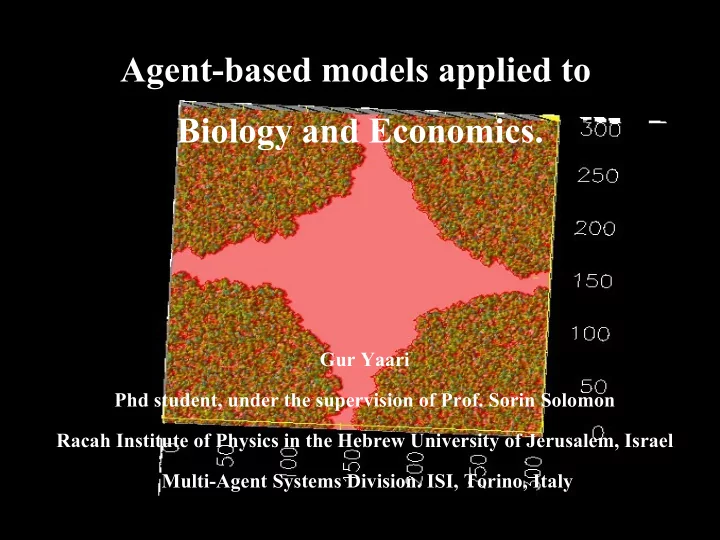
Agent-based models applied to Biology and Economics. Gur Yaari Phd student, under the supervision of Prof. Sorin Solomon Racah Institute of Physics in the Hebrew University of Jerusalem, Israel Multi-Agent Systems Division. ISI, Torino, Italy
Agent-based models applied to Biology and Economics. Gur Yaari Phd student, under the supervision of Prof. Sorin Solomon Racah Institute of Physics in the Hebrew University of Jerusalem, Israel Multi-Agent Systems Division. ISI, Torino, Italy
“G.L.V” Generalized Lotka Volterra Stochastic Lotka-Volterra Systems of Competing Auto-catalytic Agents lead Generically to Truncated Pareto Power Wealth Distribution, Truncated Levy Distribution of Market Returns, Clustered Volatility, Booms and Crashes. S. Solomon, in Decision Technologies for Computational Finance, edited by A.-P. Refenes, A. N. Burgess, and J. E. Moody (Kluwer Academic Publishers, 1998). http://xxx.lanl.gov/abs/cond-mat/9803367 Theoretical analysis and simulations of the generalized Lotka-Volterra model Ofer Malcai,1 Ofer Biham,1 Peter Richmond,2 and Sorin Solomon Phys. Rev. E 66, 031102 (2002) URL: http://link.aps.org/abstract/PRE/v66/e031102 doi:10.1103/ PhysRevE .66.031102 http://xxx.lanl.gov/PS_cache/cond-mat/pdf/0208/0208514.pdf Generalized Lotka Volterra (GLV) Models of Stock Markets S. Solomon, pp 301-322 in "Applications of Simulation to Social Sciences" , Eds: G Ballot and G Weisbuch; Hermes Science Publications 2000 http://xxx.lanl.gov/abs/cond-mat/9901250 Power laws in cities population, financimarkets and internet sites (scaling in systems with a variable number of components) Aharon Blank and Sorin Solomon Physica A 287 (1-2) (2000) pp.279-288 http://xxx.lanl.gov/abs/cond-mat/0003240 Power-law distributions and L'evy-stable intermittent fluctuations in stochastic systems of many autocatalytic elements. O. Malcai O. Biham and S. Solomon, Phys. Rev. E, 60, 1299 (1999). http://xxx.lanl.gov/abs/cond-mat/9907320
“AB Model” The importance of being discrete: Life always wins on the surface Nadav M. Shnerb, Yoram Louzoun, Eldad Bettelheim, and Sorin Solomon Proc. Natl. Acad. Sci. USA, Vol. 97, Issue 19, 10322-10324, September 12, 2000 http://xxx.lanl.gov/abs/adap-org/9912005 Adaptation of Autocatalytic Fluctuations to Diffusive Noise N. M. Shnerb, E. Bettelheim, Y. Louzoun, O. Agam, S. Solomon Phys Rev E Vol 63, No 2, 2001; http://xxx.lanl.gov/abs/cond-mat/0007097 HIV time hierarchy: winning the war while, loosing all the battles Uri Hershberg, Yoram Louzoun, Henri Atlan and Sorin Solomon Physica A: 289 (1-2) (2001) pp.178-190 ; http://xxx.lanl.gov/abs/nlin.AO/0006023 [pdf] The Emergence of Spatial Complexity in the immune System. Louzoun, Y, Solomon. S., Atlan. H., Cohen.I.R. (2001) Physica A , 297 (1-2) pp. 242-252. http://xxx.lanl.gov/html/cond-mat/0008133 Proliferation and Competition in Discrete Biological Systems Y Louzoun S Solomon, H Atlan and I R. Cohend Bulletin of Mathematical Biology Volume 65, Issue 3 , May 2003, P 375-396
Issues that had been explained (at least qualitatively) by these two models and their extensions: - The distribution of individuals in colonies (cities population) - The distribution of individuals/companies wealth - The distribution of number of individuals for various species - The distribution of word's frequency in a language -Genetic evolution – The origin of life (??) The H.I.V war against our Immune system -Patches of green vegetation in the desert - Waiting for new Ideas...
“G.L.V” Generalized Lotka Volterra Thomas Robert Malthus (1766–1834) 1798 dx dt = a ⋅ x autocatalitic proliferation: with a =birth rate - death rate exponential solution: X(t) = X(0) e a t contemporary estimations= doubling of the population every 30yrs
Pierre François Verhulst (1804-1849) way out exponential explosion: dX/dt = a X – c X 2 1838 Solution: exponential ========== saturation at X= a / c
For humans data at the time could not discriminate between: 1. exponential growth of Malthus 2. logistic growth of Verhulst But data fit on animal population: sheep in Tasmania - exponential in the first 20 years after their introduction and completely saturated after about half a century. ==> Verhulst
“G.L.V” Generalized Lotka Volterra Alfred James Lotka (March 2, 1880 - December 5, 1949) Vito Volterra (May 3, 1860 - October 11, 1940) proposed independently (Lotka-1925 , Volterra-1926) The Lotka Volterra Equations. Describes Predator-Prey Relations: dx dt = x ⋅− ⋅ y dy dt =− y ⋅− ⋅ x
Taking into account self competition (limited resources) we have: dx dt = x ⋅− 1 ⋅ x − 12 ⋅ y dy dt = y ⋅−− 1 ⋅ y 21 ⋅ x Results: Cycles in time in the number of Predator's-Prey's Number of individuals
“G.L.V” Generalized Lotka Volterra General Frame-work for various processes in Economics and Biology. The Model N agents (fix number) : N individuals (Economics) N spieces (Biology)
Update: each time step Choose individual i randomly from 1..N w j t 1 = w j t i = 1. . N ;i ≠ j N N 1 t ∑ a i , j ⋅ w j t − ∑ w i t 1 = w i t ⋅ c i , j ⋅ w j t ⋅ w i t j = 1 j = 1 Stochastic Term! t D ≡ 〈 t 2 〉 − 〈 t 〉 2 Is a stochastic variable drawn from a distribution with :
In order To Kis (keep it simple) it: one can choose uniform interaction: c i , j = a a i , j = a N N And then the process can be described by: w i t 1 = w i t ⋅ 1 t a ⋅ w t − c ⋅ w i t ⋅ w t N w t = 1 N ⋅ ∑ w i t where : j = 1
Another possibility is: w i t 1 = w i t ⋅ 1 t With the restriction: w i t ≥ c ⋅ w t
X i (t+τ) – X i (t) = λ i (t) X i (t) + a X (t) – c( X .,t) X i (t) admits a few practical interpretations X i (t) = the individual wealth of the agent i then λ i (t) = the random part of the returns that its capital X i (t) produces during the time between t and t+τ a = the autocatalytic property of wealth at the social level = the wealth that individuals receive as members of the society in subsidies, services and social benefits. This is the reason it is proportional to the average wealth This term prevents the individual wealth falling below a certain minimum fraction of the average. c( X .,t) parametrizes the general state of the economy: large and positive correspond = boom periods negative =recessions
A different interpretation: a set of companies i = 1, … , N X i (t)= shares prices ~ capitalization of the company i ~ total wealth of all the market shares of the company λ i (t) = fluctuations in the market worth of the company ~ relative changes in individual share prices (typically fractions of the nominal share price) a X = correlation between X i and the market index w c( X .,t) usually of the form c X → represents competition Time variations in global resources may lead to lower or higher values of c →increases or decreases in the total X
Yet another interpretation: investors herding behavior (also cities) X i (t)= number of traders adopting a similar investment policy or position. they comprise herd i one assumes that the sizes of these sets vary autocatalytically according to the random factor λ i (t) This can be justied by the fact that the visibility and social connections of a herd are proportional to its size a X represents the diffusion of traders between the herds c( X .,t) = popularity of the stock market as a whole competition between various herds in attracting individuals
Important Results: When N is very large and t → ∞ , The “wealth” (w's) distribution approaches a stationary distribution with the well common empirical feature of a power-law “tail”. t x i t = w i t i = 1,... n w For the first For the second case one gets: case one gets: 1 − − 1 − − 1 − ⋅ exp P x = x P x ~ x x = 1 2 ⋅ a 1 = D 1 − c
Computer's Simulations
Fits the well known empirical Pareto's law Or the Zipf's law Vilfredo Pareto (1848-1923) George Kingsley Zipf , (1902-1950) Statistics Economics Word's distribution Income distribution Cities size's distribution P(x) ~ x –1- α d x P(n) ~ n - α d n n- rank
red circles: Pareto for 400 richest people is USA blue squares: simulation results − α Zipf plot of the wealths of the investors in the Forbes 400 of 2003 vs. their ranks. The corresponding simulation results are shown in the inset. the average wealth history 88-2003 and model fit
In addition, the average of the wealth is basically a result of a random walk with steps taken from a power-law distribution → truncated Levy distribution: − 1 w t − w t r = L r = 0 ≡ P w t = w t ~ w t A strong prediction of this model is that the exponents of the wealth distribution and the returns of the stock market (the fluctuations of the average wealth ) are connected through a simple connection: 1 ⇒ 1
−1/β And indeed it was found The relative probability of empirically: the price being the same as a function of the time interval α Prediction of β The Lotka- Volterra- model: M. Levy S.S
Recommend
More recommend
Explore More Topics
Stay informed with curated content and fresh updates.

