Advanced Mathematical Methods Part II Statistics Statistical - PowerPoint PPT Presentation
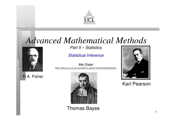
Advanced Mathematical Methods Part II Statistics Statistical Inference Mel Slater http://www.cs.ucl.ac.uk/staff/m.slater/Teaching/Statistics/ R.A. Fisher Karl Pearson Thomas Bayes 1 Outline Bayes Theorem Examples of Inference
Advanced Mathematical Methods Part II – Statistics Statistical Inference Mel Slater http://www.cs.ucl.ac.uk/staff/m.slater/Teaching/Statistics/ R.A. Fisher Karl Pearson Thomas Bayes 1
Outline � Bayes’ Theorem � Examples of Inference � Estimation � Likelihood Ratios � Classical Statistical Testing � Gallery of Standard Tests 2
Statistical Inference � To make informed probability statements about hypotheses in the light of evidence. � H 1 , H 2 , …, H n are n mutually exclusive and exhaustive ‘events’ • one and only one is true � E is some event. � Require P(H j |E) • If we had initial P(H j ) • How should the probability of H j be updated if evidence E was known to have occurred? 3
Bayes Theorem � It is easy to see: � and therefore: � and so: 4
Bayes’ Theorem and Inference � If we interpret the H j as hypotheses and E as evidence then Bayes’ Theorem gives a method for statistical inference. � P(H j ) is called the prior probability � P(E|H j ) is the likelihood � P(H j |E) is the posterior probability � posterior ∝ likelihood * prior 5
Bayes’ Theorem for Distributions � Suppose X is a r.v. with probability density dependent on a parameter set θ (e.g., mean and variance). � f( θ |x) ∝ f(x| θ ) f( θ ) • f( θ ) ~ prior probability distribution for θ • f(x| θ ) ~ the likelihood • x may be a vector of r.v.s 6
Example - ESP � Recall the ‘extra sensory hypothesis’ example and J.B. Rhine from 1930s � Simplification of the Rhine experiments: • Target person (T) is in Lab1 selecting cards at random from a pack – each card has a square or circle. • Subject (S) is in Lab2 and on signal guesses which card T is looking at and writes it down. • There is no possible communication between Lab1 and Lab2 (etc). • X = number of correct guesses subject makes in n trials. 7
Example ESP � X ~ binomial(p,n) where p = P(correct guess) � Suppose we ‘knew nothing’ about p, we would assign p ~ uniform(0,1) distribution. � We require f(p|x) : the posterior distribution of p given that we know that x correct guesses were made. 8
Example ESP ∝ − − � f(p|x) ∝ f(x|p)f(p) x n x ( | ) ( 1 ) f p x p p � This is is the Beta distribution with parameters a = x+1 and b = n-x+1 • See notes � Suppose n = 500 and x = 280. � From MATLAB (betacdf) we find • P(p > 0.5) = 0.9964 � We would conclude that something ‘beyond chance’ must be happening. � (This is the type of data that Rhine obtained again and again!). 9
Example ESP Continued � From MATLAB using betainv, we can find for this example that • P(0.5162 < p < 0.6029) = 0.95 � Since this range does not include the value of ½ which should be expected if chance alone was operating then we may decide to reject the hypothesis that this was the result of coincidence � This is called an ‘interval estimate’ for p. 10
Point Estimators � For the p ~ beta(a,b) distribution it can be shown that: + 1 x = ( | ) E p x + 2 n + − + ( 1 )( 1 ) x n x = ( | ) Var p x + + 2 ( 2 ) ( 3 ) n n � E(p|x) could serve as a single value estimator with the variance as an indication of margin of error. • E(p|x) = 0.5598 • Standard deviation(p|x) = 0.0221 11
Properties of the Estimator for p � For large n, • E(p|x) ∝ x/n • Var(p|x) → 0 • Probability and frequency ratio become identical. � Note that E((x+1)/(n+2)|p) ≠ p • This estimator is called biased. � In general if t is an estimator for parameter θ based on n observations then • E(t| θ ) = θ unbiased • Var(t| θ ) → 0 as n → ∞ consistent. 12
The Posterior Beta Distribution � The pdf shows how most of the probability is concentrated above 0.5. � The full posterior distribution is the ideal way to examine the situation. 13
Recasting as a Statistical Test � In our example we state a null hypothesis and an alternative: • H 0 : p = ½ • H 1 : p > ½ � We will decide to reject H 0 if on our ‘posterior distribution’ we find • P(p > ½ | data) > some high value, eg: • reject H 0 if • P(p > ½ | x ) > 0.95 14
Statistical Test � We know p|x ~ Beta(x+1,n-x+1) � Using MATLAB notation the test is: • Reject H 0 if • 1 – betacdf(0.5,x+1,n-x+1) > 0.95, or • betacdf(0.5,x+1,n-x+1) < 0.05 � If we find in advance a value x 0 such that • betacdf(0.5,x 0 +1,n-x 0 +1) = 0.05 � Then the test becomes • Reject H 0 if the observed X >= x 0 15
Classical Statistical Testing � The 0.05 is called the ‘significance level’ – it is equal to the prob of rejecting H 0 when in fact it is ‘true’ � The significance level is usually denoted by α = P(Type I error) � P(Type II error) = β � Power = 1- β H0 decided H1 decided H0 ‘true’ Type I error H1 ‘true’ Type II error power 16
Classical Statistical Tests � Rely on Central Limit Theorem � Testing Population Means � Testing Difference of Means � Testing Variances � Testing Ratios of Variances � Testing Goodness of Fit � Relationship between variables 17
Central Limit Theorem � See notes for ‘proof’ � X is any r.v. with finite mean µ and variance σ 2 . � x 1 ,x 2 , …, x n are n independent observations on X. n 1 ∑ = x x � The sample mean is i n = 1 i � For n ‘large’ σ 2 µ ~ ( , ) x N n 18
Central Limit Theorem � If X itself is Normal then the result is exact for any n � In practice n > 30 is usually used as the interpretation for ‘large’. � This can be illustrated very easily with simulation (see exercises). 19
Hypothesis about a Mean � X is any r.v. with finite mean µ and variance σ 2 � We assume that σ 2 is known, but that µ is unknown � The problem is to make inferences about µ from � x 1 ,x 2 , …, x n • n independent observations on X. 20
Hypothesis about a mean � Assume we know ‘nothing’ about µ � The ‘pseudo’ pdf for µ would then be • f( µ ) = k, - ∝ < µ < ∝ – This is not a true pdf! � From Bayes’ Theorem µ ∝ µ µ ( | ) ( | ) ( ) f x f x f � From the CLT we know therefore that σ 2 µ = ( | ) ( , ) f x N x n 21
Estimators for µ � An estimator for µ µ = ( | ) E x x σ 2 µ = ( | ) Var x n � From the normal distribution it is also easy to show for example that a 95% interval estimate is: 22
Hypothesis Test for µ � H 0 : µ = µ 0 � H 1 : µ = µ 1 > µ 0 sig. level here is 0.05 23
Recommend
More recommend
Explore More Topics
Stay informed with curated content and fresh updates.
