Accelerated first-order methods Geoff Gordon & Ryan Tibshirani - PowerPoint PPT Presentation
Accelerated first-order methods Geoff Gordon & Ryan Tibshirani Optimization 10-725 / 36-725 1 Remember generalized gradient descent We want to solve x R n g ( x ) + h ( x ) , min for g convex and differentiable, h convex Generalized
Accelerated first-order methods Geoff Gordon & Ryan Tibshirani Optimization 10-725 / 36-725 1
Remember generalized gradient descent We want to solve x ∈ R n g ( x ) + h ( x ) , min for g convex and differentiable, h convex Generalized gradient descent: choose initial x (0) ∈ R n , repeat: x ( k ) = prox t k ( x ( k − 1) − t k · ∇ g ( x ( k − 1) )) , k = 1 , 2 , 3 , . . . where the prox function is defined as 1 2 t � x − z � 2 + h ( z ) prox t ( x ) = argmin z ∈ R n If ∇ g is Lipschitz continuous, and prox function can be evaluated, then generalized gradient has rate O (1 /k ) (counts # of iterations) We can apply acceleration to achieve optimal O (1 /k 2 ) rate! 2
Acceleration Four ideas (three acceleration methods) by Nesterov (1983, 1998, 2005, 2007) • 1983: original accleration idea for smooth functions • 1988: another acceleration idea for smooth functions • 2005: smoothing techniques for nonsmooth functions, coupled with original acceleration idea • 2007: acceleration idea for composite functions 1 Beck and Teboulle (2008): extension of Nesterov (1983) to composite functions 2 Tseng (2008): unified analysis of accleration techniques (all of these, and more) 1 Each step uses entire history of previous steps and makes two prox calls 2 Each step uses only information from two last steps and makes one prox call 3
Outline Today: • Acceleration for composite functions (method of Beck and Teboulle (2008), presentation of Vandenberghe’s notes) • Convergence rate • FISTA • Is acceleration always useful? 4
Accelerated generalized gradient method Our problem x ∈ R n g ( x ) + h ( x ) , min for g convex and differentiable, h convex Accelerated generalized gradient method: choose any initial x (0) = x ( − 1) ∈ R n , repeat for k = 1 , 2 , 3 , . . . y = x ( k − 1) + k − 2 k + 1( x ( k − 1) − x ( k − 2) ) x ( k ) = prox t k ( y − t k ∇ g ( y )) • First step k = 1 is just usual generalized gradient update • After that, y = x ( k − 1) + k − 2 k +1 ( x ( k − 1) − x ( k − 2) ) carries some “momentum” from previous iterations • h = 0 gives accelerated gradient method 5
1.0 ● ● ● ● ● ● ● ● ● ● ● ● ● ● ● ● ● ● ● ● ● ● ● ● ● ● ● ● ● ● ● ● ● ● ● ● ● ● ● ● ● ● ● ● ● ● ● ● ● ● ● ● ● ● ● ● ● ● ● ● ● ● ● ● ● ● ● ● ● ● ● ● ● ● ● ● ● ● ● ● ● ● ● ● ● ● ● ● ● ● ● ● ● ● ● 0.5 ● (k − 2)/(k + 1) ● ● 0.0 ● −0.5 ● 0 20 40 60 80 100 k 6
Consider minimizing n � � � − y i a T i x + log(1 + exp( a T f ( x ) = i x ) i =1 i.e., logistic regression with predictors a i ∈ R p This is smooth, and ∇ f ( x ) = − A T ( y − p ( x )) , where p i ( x ) = exp( a T i x ) / (1 + exp( a T i x )) for i = 1 , . . . n No nonsmooth part here, so prox t ( x ) = x 7
Example (with n = 30 , p = 10 ): 1e+01 Gradient descent Accelerated gradient 1e+00 1e−01 f(k)−fstar 1e−02 1e−03 0 20 40 60 80 100 k 8
Another example ( n = 30 , p = 10 ): Gradient descent Accelerated gradient 1e−01 f(k)−fstar 1e−03 1e−05 0 20 40 60 80 100 k Not a descent method! 9
Reformulation Initialize x (0) = u (0) , and repeat for k = 1 , 2 , 3 , . . . y = (1 − θ k ) x ( k − 1) + θ k u ( k − 1) x ( k ) = prox t k ( y − t k ∇ g ( y )) u ( k ) = x ( k − 1) + 1 ( x ( k ) − x ( k − 1) ) θ k with θ k = 2 / ( k + 1) This is equivalent to the formulation of accelerated generalized gradient method presented earlier (slide 5). Makes convergence analysis easier (Note: Beck and Teboulle (2008) use a choice θ k < 2 / ( k + 1) , but very close) 10
Convergence analysis As usual, we are minimizing f ( x ) = g ( x ) + h ( x ) assuming • g is convex, differentiable, ∇ g is Lipschitz continuous with constant L > 0 • h is convex, prox function can be evaluated Theorem: Accelerated generalized gradient method with fixed step size t ≤ 1 /L satisfies f ( x ( k ) ) − f ( x ⋆ ) ≤ 2 � x (0) − x ⋆ � 2 t ( k + 1) 2 Achieves the optimal O (1 /k 2 ) rate for first-order methods! I.e., to get f ( x ( k ) ) − f ( x ⋆ ) ≤ ǫ , need O (1 / √ ǫ ) iterations 11
Helpful inequalities We will use 1 − θ k 1 ≤ , k = 1 , 2 , 3 , . . . θ 2 θ 2 k k − 1 We will also use h ( v ) ≤ h ( z ) + 1 t ( v − w ) T ( z − v ) , all z, w, v = prox t ( w ) Why is this true? By definition of prox operator, v minimizes 1 0 ∈ 1 2 t � w − v � 2 + h ( v ) ⇔ t ( v − w ) + ∂h ( v ) − 1 ⇔ t ( v − w ) ∈ ∂h ( v ) Now apply definition of subgradient 12
Convergence proof We focus first on one iteration, and drop k notation (so x + , u + are updated versions of x, u ). Key steps: • g Lipschitz with constant L > 0 and t ≤ 1 /L ⇒ g ( x + ) ≤ g ( y ) + ∇ g ( y ) T ( x + − y ) + 1 2 t � x + − y � 2 • From our bound using prox operator, h ( x + ) ≤ h ( z ) + 1 t ( x + − y ) T ( z − x + ) + ∇ g ( y ) T ( z − x + ) all z • Adding these together and using convexity of g , f ( x + ) ≤ f ( z ) + 1 t ( x + − y ) T ( z − x + ) + 1 2 t � x + − y � 2 all z 13
• Using this bound at z = x and z = x ∗ : f ( x + ) − f ( x ⋆ ) − (1 − θ )( f ( x ) − f ( x ⋆ )) ≤ 1 t ( x + − y ) T ( θx ⋆ + (1 − θ ) x − x + ) + 1 2 t � x + − y � 2 = θ 2 � � u − x ⋆ � 2 − � u + − x ⋆ � 2 � 2 t • I.e., at iteration k , t ( f ( x ( k ) ) − f ( x ⋆ )) + 1 2 � u ( k ) − x ⋆ � 2 θ 2 k ≤ (1 − θ k ) t ( f ( x ( k − 1) ) − f ( x ⋆ )) + 1 2 � u ( k − 1) − x ⋆ � 2 θ 2 k 14
• Using (1 − θ i ) /θ 2 i ≤ 1 /θ 2 i − 1 , and iterating this inequality, t ( f ( x ( k ) ) − f ( x ⋆ )) + 1 2 � u ( k ) − x ⋆ � 2 θ 2 k ≤ (1 − θ 1 ) t ( f ( x (0) ) − f ( x ⋆ )) + 1 2 � u (0) − x ⋆ � 2 θ 2 1 = 1 2 � x (0) − x ⋆ � 2 • Therefore f ( x ( k ) ) − f ( x ⋆ ) ≤ θ 2 2 2 t � x (0) − x ⋆ � 2 = t ( k + 1) 2 � x (0) − x ⋆ � 2 k 15
Backtracking line search A few ways to do this with acceleration ... here’s a simple method (more complicated strategies exist) First think: what do we need t to satisfy? Looking back at proof with t k = t ≤ 1 /L , • We used g ( x + ) ≤ g ( y ) + ∇ g ( y ) T ( x + − y ) + 1 2 t � x + − y � 2 • We also used (1 − θ k ) t k ≤ t k − 1 , θ 2 θ 2 k − 1 k so it suffices to have t k ≤ t k − 1 , i.e., decreasing step sizes 16
Backtracking algorithm: fix β < 1 , t 0 = 1 . At iteration k , replace x update (i.e., computation of x + ) with: • Start with t k = t k − 1 and x + = prox t k ( y − t k ∇ g ( y )) • While g ( x + ) > g ( y ) + ∇ g ( y ) T ( x + − y ) + 2 t k � x + − y � 2 , 1 repeat: ◮ t k = βt k and x + = prox t k ( y − t k ∇ g ( y )) Note this achieves both requirements. So under same conditions ( ∇ g Lipschitz, prox function evaluable), we get same rate Theorem: Accelerated generalized gradient method with back- tracking line search satisfies f ( x ( k ) ) − f ( x ⋆ ) ≤ 2 � x (0) − x ⋆ � 2 t min ( k + 1) 2 where t min = min { 1 , β/L } 17
FISTA Recall lasso problem, 1 2 � y − Ax � 2 + λ � x � 1 min x and ISTA (Iterative Soft-thresholding Algorithm): x ( k ) = S λt k ( x ( k − 1) + t k A T ( y − Ax ( k − 1) )) , k = 1 , 2 , 3 , . . . S λ ( · ) being matrix soft-thresholding. Applying acceleration gives us FISTA (F is for Fast): 3 v = x ( k − 1) + k − 2 k + 1( x ( k − 1) − x ( k − 2) ) x ( k ) = S λt k ( v + t k A T ( y − Av )) , k = 1 , 2 , 3 , . . . 3 Beck and Teboulle (2008) actually call their general acceleration technique (for general g, h ) FISTA, which may be somewhat confusing 18
Lasso regression: 100 instances (with n = 100 , p = 500 ): 1e+00 1e−01 f(k)−fstar 1e−02 1e−03 ISTA 1e−04 FISTA 0 200 400 600 800 1000 k 19
Lasso logistic regression: 100 instances ( n = 100 , p = 500 ): 1e+00 1e−01 f(k)−fstar 1e−02 1e−03 ISTA 1e−04 FISTA 0 200 400 600 800 1000 k 20
Is acceleration always useful? Acceleration is generally a very effective speedup tool ... but should it always be used? In practice the speedup of using acceleration is diminished in the presence of warm starts . I.e., suppose want to solve lasso problem for tuning parameters values λ 1 ≥ λ 2 ≥ . . . ≥ λ r • When solving for λ 1 , initialize x (0) = 0 , record solution ˆ x ( λ 1 ) • When solving for λ j , initialize x (0) = ˆ x ( λ j − 1 ) , the recorded solution for λ j − 1 Over a fine enough grid of λ values, generalized gradient descent perform can perform just as well without acceleration 21
Sometimes acceleration and even backtracking can be harmful! Recall matrix completion problem: observe some only entries of A , ( i, j ) ∈ Ω , we want to fill in the rest, so we solve 1 2 � P Ω ( A ) − P Ω ( X ) � 2 min F + λ � X � ∗ X where � X � ∗ = � r i =1 σ i ( X ) , nuclear norm, and � X ij ( i, j ) ∈ Ω [ P Ω ( X )] ij = 0 ( i, j ) / ∈ Ω Generalized gradient descent with t = 1 (soft-impute algorithm): updates are X + = S λ ( P Ω ( A ) + P ⊥ Ω ( X )) where S λ is the matrix soft-thresholding operator ... requires SVD 22
Recommend
More recommend
Explore More Topics
Stay informed with curated content and fresh updates.


