Ab initio methods: how/why do they work D.Svergun Small-angle - PDF document

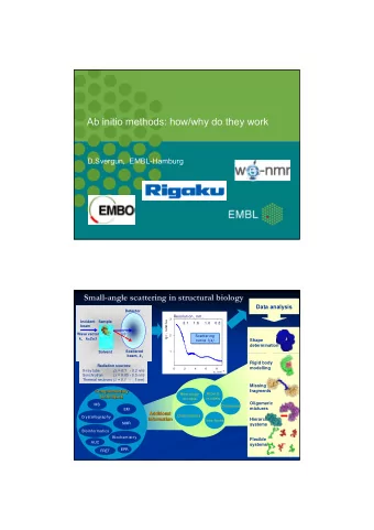
29-Oct-14 Ab initio methods: how/why do they work D.Svergun Small-angle scattering in structural biology Data analysis Detector Resolution, nm: 3 Incident Sample lg I, relative 3.1 1.6 1.0 0.8 beam Wave vector 2 θ 2 Scattering k, k=2  /  Shape curve I(s) determination Scattered Solvent 1 beam, k 1 Rigid body Radiation sources: modelling 0 2 4 6 8 X-ray tube (  = 0.1 - 0.2 nm) s, nm -1 Synchrotron (  = 0.05 - 0.5 nm) Thermal neutrons (  = 0.1 - 1 nm) Missing fragments Complementary Homology Atomic techniques models models Oligomeric MS Distances mixtures EM Additional Orientations Crystallography information Hierarchical Interfaces NMR systems Bioinformatics Biochemistry Flexible AUC systems EPR FRET 1

29-Oct-14 Major problem for biologists using SAS • In the past, many biologists did not believe that SAS yields more than the radius of gyration • Now, an immensely grown number of users are attracted by new possibilities of SAS and they want rapid answers to more and more complicated Questions • The users often have to perform numerous cumbersome actions during the experiment and data analysis, to become each of the Answers Now we shall go through the major steps required on the way Step 1: know, which units are used The momentum transfer Resolution, nm: 3 lg I, relative 3.1 1.6 1.0 0.8 [q, Q, s, h, μ, κ …] = 4π sin(θ)/λ, I(s)=I 0 *exp(-sR g /3), sR g <1.3 2 Scattering curve I(s) 1 [s, S, k, … ] = 2 sin(θ)/λ I(s)=I 0 *exp(-2πsR g /3), sR g <1.3*2π 0 2 4 6 8 s, nm -1 GNOM or CRYSOL input: Angular units in the input file: 4*pi*sin(theta)/lambda [1/angstrom] (1) 4*pi*sin(theta)/lambda [1/nm] (2) 2 * sin(theta)/lambda [1/angstrom] (3) 2 * sin(theta)/lambda [1/nm] (4) 2

29-Oct-14 Scattering from dilute macromolecular solutions (monodisperse systems) D sin sr    ( ) 4 ( ) I s p r dr sr 0 The scattering is proportional to that of a single particle averaged over all orientations, which allows one to determine size, shape and internal structure of the particle at low ( 1-10 nm ) resolution. Sample and buffer scattering 3

29-Oct-14 Overall parameters Radius of gyration R g (Guinier, 1939) 1   2 2 0 exp( I(s) I( ) R s ) 3 g Molecular mass (from I(0)) Maximum size D max : p(r)=0 for r> Dmax Excluded particle volume (Porod, 1952)      2 2 V 2 I(0)/Q; ( ) Q s I s ds 0 The scattering is related to the shape (or low resolution structure) Solid sphere lg I(s), relative lg I(s), relative lg I(s), relative lg I(s), relative lg I(s), relative 0 0 0 0 0 -1 -1 -1 -1 -1 Hollow sphere -2 -2 -2 -2 -2 -3 -3 -3 -3 -3 -4 -4 -4 -4 -4 -5 -5 -5 -5 -5 -6 -6 -6 -6 -6 0.0 0.1 0.2 0.3 0.4 0.5 0.0 0.0 0.0 0.0 0.1 0.1 0.1 0.1 0.2 0.2 0.2 0.2 0.3 0.3 0.3 0.3 0.4 0.4 0.4 0.4 0.5 0.5 0.5 0.5 Dumbbell s, nm -1 s, nm -1 s, nm -1 s, nm -1 s, nm -1 Flat disc Long rod 4

29-Oct-14 Shape determination: how? Trial-and-error 3D search model M parameters 1D scattering data Non-linear search Lack of 3D information inevitably leads to ambiguous interpretation, and additional information is always required Ab initio methods Advanced methods of SAS data analysis employ spherical harmonics (Stuhrmann, 1970) instead of Fourier transformations 5

29-Oct-14 The use of spherical harmonics SAS intensity is I(s) = <I( s )>  = <{F [  ( r )]} 2 >  , where F denotes the Fourier transform, <>  stands for the spherical average, and s=( s ,  ) is the scattering vector. Expanding  ( r ) in spherical harmonics  l       ( r ) ( ) ( ) r Y lm lm  0   l m l the scattering intensity is expressed as  l 2 2     2 I s ( ) A ( ) s lm   0 l m l where the partial amplitudes A lm (s) are the Hankel transforms from the radial functions  2  2  l  A ( ) s i ( ) ( r j sr r dr )  lm lm l 0 and j l (sr) are the spherical Bessel functions. Stuhrmann, H.B. Acta Cryst., A26 (1970) 297. Structure of bacterial virus T7 Cryo-EM, 2005 SAXS, 1982 Pro-head Mature virus Agirrezabala, J. M. et al. & Carrascosa J.L. (2005) EMBO J. Svergun, D.I., Feigin, L.A. & Schedrin, B.M. 24 , 3820 (1982) Acta Cryst. A38 , 827 6

29-Oct-14 Shape parameterization by spherical harmonics Homogeneous particle Scattering density in spherical coordinates (r,  ) = (r,  ,  ) may be described by the  envelope function: r     1 , 0 ( ) r F   r ( )    0 , ( )  r F F(  ) is an Shape parameterization by a limited series of spherical harmonics: envelope function l L         ( ) ( ) ( ) F F f Y lm lm Y lm (  ) – orthogonal spherical harmonics, L l  0 m   l f lm – parametrization coefficients, Small-angle scattering intensity from the entire particle is calculated as the sum of scattering from partial harmonics: Stuhrmann, H. B. (1970) Z. l Physik. Chem. Neue Folge 72, L   2 2   ( ) 2 ( ) 177-198. I s A s lm theor    l 0 m l Svergun, D.I. et al . (1996) Acta Crystallogr. A52, 419-426. Shape parameterization by spherical harmonics Homogeneous particle  + + r + = + f 00 - f 11 A 00 (s) A 11 (s) F(  ) is an + envelope function + + + - - + +… f 20 f 22 - + A 20 (s) A 22 (s) π   R Spatial resolution: , R – radius of an equivalent sphere.  ( 1 ) L Number of model parameters f lm is ( L +1) 2 . One can easily impose symmetry by selecting appropriate harmonics in the sum. This significantly reduces the number of parameters describing F(  ) for a given L . 7

29-Oct-14 Program SASHA Bead (dummy atoms) model A sphere of radius D max is filled by Vector of model parameters: densely packed beads of radius  r 0 << D max 1 if particle Position ( j ) = x ( j ) =   0 if solvent Particle Solvent (phase assignments) Number of model parameters M  (D max / r 0 ) 3  10 3 is too big for conventional minimization methods – Monte-Carlo like approaches are to be used But: This model is able to describe rather complex shapes Chacón, P. et al. (1998) Biophys. J. 74, 2r 0 2760-2775. D max Svergun, D.I. (1999) Biophys. J. 76, 2879-2886 8

29-Oct-14 Finding a global minimum Pure Monte Carlo runs in a danger to be trapped into a local minimum Solution: use a global minimization method like simulated annealing or genetic algorithm Local and global search on the Great Wall Local search always goes to a better point and can thus be trapped in a local minimum Pure Monte-Carlo search always goes to the closest local minimum (nature: rapid quenching and vitreous ice formation) To get out of local minima, global search must be able to (sometimes) go to a worse point Slower annealing allows to search for a global minimum (nature: normal, e.g. slow freezing of water and ice formation) 9

29-Oct-14 Simulated annealing Aim: find a vector of M variables {x} minimizing a function f(x) 1. Start from a random configuration x at a “high” temperature T . Make a small step (random modification of the configuration) x  x’ and 2. compute the difference  = f(x’) - f(x) . If  < 0 , accept the step; if  > 0 , accept it with a probability e -  /T 3. 4. Make another step from the old (if the previous step has been rejected) or from the new (if the step has been accepted) configuration. Anneal the system at this temperature, i.e. repeat steps 2-4 “many” 5. (say, 100M tries or 10M successful tries, whichever comes first) times, then decrease the temperature (T’ = cT, c<1). Continue cooling the system until no improvement in f(x) is observed. 6. Shape determination: M≈ 10 3 variables (e.g. 0 or 1 bead assignments in DAMMIN Rigid body methods: M≈ 10 1 variables (positional and rotational parameters of the subunits) f(x) is always (Discrepancy + Penalty) Ab initio program DAMMIN Using simulated annealing, finds a compact dummy atoms configuration X that fits the scattering data by minimizing   2   ( ) [ ( ), ( , )] ( ) f X I s I s X P X exp where  is the discrepancy between the experimental and calculated curves, P(X) is the penalty to ensure compactness and connectivity,  > 0 its weight. compact loose disconnected 10

29-Oct-14 Why/how do ab initio methods work The 3D model is required not only to fit the data but also to fulfill (often stringent) physical and/or biochemical constrains Why/how do ab initio methods work The 3D model is required not only to fit the data but also to fulfill (often stringent) physical and/or biochemical constrains 11

29-Oct-14 A test ab initio shape determination run Program Slow mode DAMMIN Bovine serum albumin, molecular mass 66 kDa, no symmetry imposed A test ab initio shape determination run Program Slow mode DAMMIN Bovine serum albumin: comparison of the ab initio model with the crystal structure of human serum albumin 12