A wildland fire modeling and visualization environment Jan Mandel, - PowerPoint PPT Presentation
A wildland fire modeling and visualization environment Jan Mandel, University of Colorado, Denver, CO; and J. D. Beezley, A. Kochanski, V. Y. Kondratenko, L. Zhang, E. Anderson, J. Daniels II, C. T. Silva, and C. Johnson Acknowledgements Janice
A wildland fire modeling and visualization environment Jan Mandel, University of Colorado, Denver, CO; and J. D. Beezley, A. Kochanski, V. Y. Kondratenko, L. Zhang, E. Anderson, J. Daniels II, C. T. Silva, and C. Johnson
Acknowledgements • Janice Coen, Ned Patton, John Michalakes, NCAR • Eric Jorgensen, Bigyan Muherjee, Mavin Martin, Paul Rosen, University of Utah • Craig Clements, San Jose State University • Bedrich Sousedik, now at Univ. of Southern California • Nina Dobrinkova, Georgi Jordanov, Bulgarian Academy of Sciences • Barry Lynn and Guy Kelman, Weather ‐ It ‐ Is, LTD • NSF grant ATM ‐ 0835579 • NIST Fire Research Grants Program 60NANB7D6144 • NSF grant CNS ‐ 0821794 (Janus supercomputer)
OpenWFM.org components • 2D fire spread model coupled with WRF • A code with a subset of features is distributed with WRF release as WRF ‐ Fire. • The current development version available on openwfm.org as WRF coupled with SFIRE. • Extended WRF Preprocessing System (WPS) • Wiki: guides, links to software repositories • Utilities – Visualization, Data preprocessing, Diagnostics • Web interfaces, data assimilation (future)
Objectives and design limitations • Model faster than real time – Fast enough for forecasting at 100m atmosphere and 10m fire scale – Fire parameterization to capture essential fire behavior and feedback on the atmosphere • Open source, collaborative development – Public read access to source code repositories – Invite collaborations • Subject to WRF programming conventions for WRF release – Affects the choice of algorithms • Data assimilation – Modify the state (atmosphere, fire position,…) and parameters (fuels, spread rate,…) of the running coupled model in response to data – This is the overall goal but we had to have a suitable model first.
http://www.openwfm.org/wiki/List_of_SFIRE_pages
Origins • USDA Forest Service wildfire modeling system: BEHAVE ‐ fire properties at one point, FARSITE ‐ surface fire spread • NCAR’s Coupled Atmosphere ‐ Wildland Fire Enviroment (CAWFE), based on the Clark ‐ Hall research weather code, fire propagation by tracers • The Weather Research and Forecasting model (WRF) – A standard, well structured, extensible, massively parallel, and evolving – Supported , community code – Preprocessing for standard meteorological data – Built ‐ in export/import of state – essential for data assimilation! • Fire spread model by the level set method – Supports BEHAVE fire spread formulas – Flexible for easy implementation of various features – The fire location can be changed by a modifying gridded array – no tracers – Better suited for data assimilation
Representation of the fire area by a level set function • The level set function is given on center nodes of the fire mesh • Interpolated linearly, parallel to the mesh lines • Fireline connects the points where the interpolated values are zero
Evolving the fireline by the level set method Level set function L Fire area: L< 0 ∂ L = − ∇ Level set equation || || R L ∂ t Right-hand side < 0 → Level set function goes down → fire area grows
The fire model: fuel consumption fuel ignition time Time constant of fuel: 30 sec - Grass burns quickly 1000 sec – Dead & down branches(~40% decrease in mass over 10 min)
Coupling with ∂Φ = ( ) Φ R ∂ t WRF ‐ ARW Δ ( ) t R Φ = Φ + Φ * t t 3 Δ ( ) t R Φ = Φ + Φ ** * t • WRF ‐ ARW is explicit 2 ( ) in time – short time Φ +Δ = Φ + Δ Φ ** t t t tR step needed Runge-Kutta order 3 integration in time • Fire is a physics package, called only in the last Runge ‐ Atmosphere Kutta substep Heat and vapor Wind, moisture • Fire module inputs fluxes wind, outputs heat Surface fire and vapor flux
Wind interpolation • Spread rates for different fuels depend on wind at different heights • Interpolation to 6m from ideal logarithmic profile, then apply BEHAVE wind reduction factors to fuel ‐ dependent heights. – But this throws away information if there are WRF levels under 6m. • Better: Interpolate the horizontal wind to the appropriate heights from the WRF mesh directly – Exact if the wind profile is exactly logarithmic (just like piecewise linear interpolation is exact for linear functions) – If there are no WRF nodes under 6m, mathematically equivalent to the reduction factors – Tricky • The heights of the nodes are computed from the geopotential, a part of the solution • The geopotential varies a lot above the fire • The atmospheric and fire mesh have different resolutions • The result depends on the roughness length. • Take the roughness length from LANDUSE or fuels?
Software Structure WRF : add tendencies WRF : call sfire_driver wind heat and moisture tendencies Driver : get grid variables, get flags, interpolation calls, Atm : one tile: temperature and OpenMP loops, DM halos moisture tendencies from heat fluxes Model : one time step, one tile: winds in, heat fluxes out Phys : sensible and latent heat fluxes from fuel loss, fire rate of spread Core : time step for the level set equation, compute fuel loss. Dimensionless. Util : interpolation, WRF stubs, debug I/O,… WRF : error messages, log messages, constants,…
Standalone fire code MAIN Model : one time step, one tile: winds in, heat fluxes out Phys : sensible and latent heat fluxes from fuel loss, fire rate of spread Core : time step for the level set equation, compute fuel loss. Dimensionless. Util : interpolation, WRF stubs, debug I/O,… Wrf_fakes : error messages, log messages, constants,…
WRF parallel infrastructure • Distributed memory (DM): halo exchanges between grid MPI patches : each patch runs in one MPI process; patch programmer only lists the variables to exchange halo • Shared memory (SM): OpenMP loops over tiles within the patch • Computational routines are tile tile callable . They can read from a layer of cells beyond the tile but must avoid race OpenMP threads, conditions: no writing into an multicore array that another tile may read a boundary layer from Example: 2 MPI processes 4 threads each Compliance affects the choice of numerical algorithms!
Parallelism in WRF ‐ Fire: implementing a PDE solver in the WRF physics layer, meant for pointwise calculations
Diagnostic outputs • Heat flux (reaction intensity) (J/m 2 /s) • Rate of spread (m/s) • Fireline intensity – Byram(J/m/s) – new fireline intensity (J/m/s 2 ) • For the actual fire modeled: at the fireline only • For a fire danger rating : everywhere, with the rate of spread taken as the maximum rate in any direction.
Fireline intensity Byram’s: heat per unit length of the fireline from all available fuel 1m burning in 1s, regardless how far, does not depend on the speed of burning (J/m/s) 2 spread rate (m / s)* heat contents of fuel (J/kg)*available fuel (kg/m ) New: heat per unit length of the fireline from the newly burning 1m fuel only the fireline moves over in a small unit of time ( J/m/s 2 ) 2 1 spread rate (m / s)* heat contents of fuel (J/kg)* available fuel (kg/m ) 2 burn time (s)
Walk ‐ through desktop client: VisTrails/VisMashups • Simplified development of user interfaces inVisTrails • save simulation, data, process, and user settings as a workflow
Web ‐ based interface: CrowdLabs • VisMashups on the web • Integrates social web site and scalable evironment to collaboratively analyze and visualize data • For now, from stored simulations • Future: communicate with a supercomputing server to run simulations
Web ‐ based interface: Google Earth and Google Maps • The same KML files display in both • A de ‐ facto standard for wildland fire information • Simulation layer combines with other information (perimeter, images,…) – Animation in Google Maps – Manually advanced frames and a fly ‐ through in Google Earth • Near future: start and control simulation on a supercomputing server, use automatically retrieved fuel, topography, and meteorological data
Web ‐ based interface: Google Maps
Fire heat flux in Google Earth
Simulation of the FireFlux experiment (Clements et al. 2007) Visualization in VAPOR by Bedrich Sousedik
25 2007 Witch fire Model Setup � Atmospheric domains: D01 D01 120x96 32km resolution D02 121x97 10.6km resolution D03 126x103 3.5km resolution D02 D04 135x94 1.18km resolution D03 D04 D05 155x118 390m resolution D05 � Fire model Nested in D05 3100x2360 , 19.5m resolution
2007 Witch fire burned area
2007 Witch fire 27 WRF Fire perimeter (blue) observed fire perimeter (black) D01 D02 D03 D04 D05
Current and future directions • Web ‐ based interfaces to run simulations • Data assimilation • Case studies, validation • Fire code improvements • Rothermel/BEHAVE calibrated spread rates include the feedback from the atmosphere; ours should not • Scale dependence, role of the feedback on the atmosphere,…
Recommend
More recommend
Explore More Topics
Stay informed with curated content and fresh updates.
