A Second-Order Model of the Stock Market Robert Fernholz INTECH - PowerPoint PPT Presentation
A Second-Order Model of the Stock Market Robert Fernholz INTECH Conference in honor of Ioannis Karatzas Columbia University, New York June 48, 2012 This is joint research with T. Ichiba, I. Karatzas. Introduction A first-order model for a
A Second-Order Model of the Stock Market Robert Fernholz INTECH Conference in honor of Ioannis Karatzas Columbia University, New York June 4–8, 2012 This is joint research with T. Ichiba, I. Karatzas.
Introduction A first-order model for a stock market is a model that assigns to each stock in the market a return parameter and a variance parameter that depend only on the rank of the stock. A second-order model for a stock market is a model that assigns these parameters based on both the rank and the name of the stock. A second-order model is an example of a hybrid Atlas model. Acknowledgements. The speaker thanks Adrian Banner, Daniel Fernholz, Vassilios Papathanakos, and Johannes Ruf for their many helpful discussions and suggestions, as well as for their participation and inspiration during the course of this research.
Reference I R. Fernholz, T. Ichiba, and I. Karatzas (2012). A second-order stock market model. Annals of Finance, to appear.
Stock markets A market is a family of stocks X = ( X 1 , . . . , X n )represented by positive absolutely continuous semimartingales defined on [ 0 , 1 ) or on R . The value X i ( t ) of the stock X i at time t represents the total capitalization of the company at that time. Let Z represent the total capitalization of the market, Z ( t ) , X 1 ( t ) + · · · + X n ( t ) . Then the market weights µ i , for i = 1 , . . . , n , given by µ i ( t ) , X i ( t ) Z ( t ) , define the market portfolio µ .
Market stability We shall assume that the market weight process µ = ( µ 1 , . . . , µ n ) has a stable, or steady-state, distribution, and that the system is in that stable distribution. We shall be interested in the relative behavior of the log-capitalizations or log-weights. If µ ( t ) is in its steady-state distribution, then the log-di ff erence processes defined by log X i ( t ) � log X j ( t ) = log µ i ( t ) � log µ j ( t ) , for i , j = 1 , . . . , n , will also be in their steady-state distribution. We shall also assume that there are almost surely no triple points for the market, i.e., there is no time t at which X i ( t ) = X j ( t ) = X k ( t ) for i < j < k , almost surely.
Ranked processes Consider the ranked capitalization processes X (1) ( t ) � · · · � X ( n ) ( t ) , and the corresponding ranked market weights µ (1) ( t ) � · · · � µ ( n ) ( t ) . Let r t ( i ) represent the rank of X i ( t ), and let p t be the inverse permutation of r t , so X i ( t ) = X ( r t ( i )) ( t ) and X ( k ) ( t ) = X p t ( k ) ( t ) . The ranked market weights ( µ (1) ( t ) , . . . , µ ( n ) ( t )) comprise the capital distribution curve of the market at time t .
Capital distribution curve 1e − 01 1e − 03 WEIGHT 1e − 05 1e − 07 1 5 10 50 100 500 1000 5000 RANK Capital distribution of the U.S. market: 1929–1999.
First-order models A first-order model is a stock market model defined by d log b X i ( t ) = g ˆ r t ( i ) dt + � ˆ r t ( i ) dW i ( t ) , for i = 1 , . . . , n , where g 1 , . . . , g n are constants, � 1 , . . . , � n are positive constants, and W = ( W 1 , . . . , W n ) is a Brownian motion. We shall assume that the g k satisfy g 1 + · · · + g n = 0 , and X m g k < 0 , k =1 for m < n . With these parameters, the b X i form an asymptotically stable system.
Rank-based parameters Suppose we have a market X that is in its steady-state distribution. We define the asymptotic rank-based relative variances for the market by h µ p t ( k ) i ( t ) σ 2 k , lim , t t !1 and the asymptotic rank-based relative growth rates by Z T 1 g k , lim d log µ p t ( k ) ( t ) . T T !1 0 Since these parameters are based on the market weight processes µ i , the parameters represent values measured relative to the market capitalization process X .
Rank-based variances 0.4 0.3 VARIANCE RATE 0.2 0.1 0.0 0 1000 2000 3000 4000 5000 RANK σ 2 k for U.S. market: 1990–1999.
Local times for the rank processes Let Λ k , k +1 be the local time of log( µ ( k ) /µ ( k +1) ) � 0 at the origin. Then d log µ ( k ) ( t ) = d log µ p t ( k ) ( t ) + 1 2 d Λ k , k +1 ( t ) � 1 2 d Λ k � 1 , k ( t ) . For k = 1 , . . . , n � 1, we can define the asymptotic local time t !1 t � 1 Λ k , k +1 ( t ) , λ k , k +1 , lim and let λ 0 , 1 = 0 = λ n , n +1 . It can be shown that � � g k = 1 λ k � 1 , k � λ k , k +1 , 2 for k = 1 , . . . , n , and it follows that g 1 + · · · + g n = 0.
Relative growth rates 0.02 0.00 VARIANCE RATE -0.02 -0.04 -0.06 0 1000 2000 3000 4000 5000 RANK Normalized g k for U.S. market: 1990–1999.
A first-order market model The first-order model with d log b X i ( t ) = g ˆ r t ( i ) dt + σ ˆ r t ( i ) dW i ( t ) , is called the first-order model for the market X . As we have seen, the growth and variance parameters for the b X i are derived from the relative growth and variance parameters corresponding to the market weight processes µ i , not directly from the price processes X i . The steady-state capital distribution curve for the first-order model of the stock market will be about the same as the capital distribution curve for the market itself.
Mathematical characteristics of first-order models I A first-order model is asymptotically stable. I A first-order model may have triple points where X i ( t ) = b b X j ( t ) = b X k ( t ) for i < j < k , but the local time at the origin for log( b X ( k ) / b X ( ` ) ) � 0 is zero if ` > k + 1. I A first-order model is ergodic in the sense that Z T 1 X ( k ) ( t ) } dt = 1 lim n . 1 { b X i ( t )= b T T !1 0 This ergodicity does not seem reasonable for a real market, so we must extend our model.
Hybrid models A hybrid (Atlas) model is a stock market model defined by d log b X i ( t ) = ( � i + g ˆ r t ( i ) ) dt + � i , ˆ r t ( i ) dW i ( t ) , for i = 1 , . . . , n , with constants g k , � i and � ik > 0, for i , k = 1 , . . . , n , and a Brownian motion W . These parameters satisfy n n X X g k = � i = 0 , k =1 i =1 and, for any permutation ⇡ 2 Σ n , m X ( g k + � ⇡ ( k ) ) < 0 , for m < n . k =1 We shall use first-order variances, so � 2 ik = � 2 k for all i and k .
Occupation rates For a market X , the expected occupation rate Z T 1 ✓ ki , lim 1 { X i ( t )= X ( k ) ( t ) } dt T T !1 0 is defined for all i and k . The matrix ✓ = ( ✓ ki ) is bistochastic, and we shall assume that all the entries are positive. For a hybrid model b X with occupation-rate matrix ˆ ✓ , X n ˆ ˆ g k = g k + ✓ ki � i i =1 n X ˆ 0 = � i + ✓ ki g k , k =1 where the ˆ g k are the rank-based relative growth rates.
Parameter estimates based on occupation rates In matrix form, this can be expressed g = g + ˆ ˆ ✓� 0 = � + ˆ ✓ T g , where � , g , and ˆ g are column vectors. From this we see that � = � ˆ ✓ T g , (1) so � ✓ T � I n � ˆ ✓ ˆ ˆ g = g . (2) As we have seen, ˆ g can be estimated directly, so we need to solve (2) for g , and then � can be calculated using (1).
Second-order parameter estimation Let ✓ be the occupation-rate matrix of the market X . Since ✓ is bistochastic with positive entries, so are ✓ T and ✓✓ T . By the Perron-Frobenius theorem, ✓✓ T will have a simple eigenvalue equal to 1 with eigenvector e 1 = (1 , 1 , . . . , 1) 0 , and all the other eigenvalues will have absolute value less than 1 (see Perron, O. (1907) Zur Theorie der Matrices, Math. Annalen 64, 248–263). From this it follows that I n � ✓✓ T has rank n � 1, and its kernel is generated by e 1 , so the condition that the g k sum to zero ensures a unique solution to � I n � ✓✓ T � g = g .
Exploratory second-order parameter estimation Unfortunately, it seems to be impossible to estimate ✓ , so although we can use it to prove the existence and uniqueness of g , we cannot actually solve the equations. Instead, we plan to work with X n g k = g k + ✓ ki � i i =1 in such a way that we can solve for the g k recursively. Once we have found g and g , we then can estimate � directly by using Z T � � 1 � i = lim d log µ i ( t ) � g r t ( i ) dt . T T !1 0
Time reversal and parameter estimation Let X be a stable market defined for t 2 R . We can define the time-reversed market e X with price processes e X i ( t ) , X i ( � t ) and weight processes e µ i ( t ) = µ i ( � t ). Then: I The forward and backward occupation rates ✓ ki are equal. I The forward and backward asymptotic local times λ k are equal (see, e.g., Bertoin, J. (1987) Temps locaux et int´ egration stochastique pour les processus de Dirichlet, S´ eminaire de Probabilit´ es (Strasbourg) 21, 191–205). I Hence, the forward and backward g k are equal. I Hence, the forward and backward g k are equal. I Hence, the forward and backward � i are equal. I Quadratic-variation is invariant under time reversal.
Market flow The forward flow ' k of the market X at rank k in the market is defined for ⌧ 2 [ 0 , 1 ) by Z T ⇣ µ p t ( k ) ( t + ⌧ ) ⌘ 1 ' k ( ⌧ ) , lim log dt . T µ ( k ) ( t ) T !1 0 The backward flow e ' k of the market is defined by Z T ⇣e ⌘ µ p t ( k ) ( t + ⌧ ) 1 ' k ( ⌧ ) , lim e log dt . T µ ( k ) ( t ) e T !1 0 The forward and backward flows need not be equal.
Forward and backward flow for top 250 stocks 2.00 1.00 0.50 0.20 % 0.10 0.05 0.02 0 200 400 600 800 1000 DAYS µ ( k ) (0) e ' k ( ⌧ ) (black), µ ( k ) (0) e e ' k ( ⌧ ) (red): 1990–1999.
Recommend
More recommend
Explore More Topics
Stay informed with curated content and fresh updates.
