A prior near-ignorance Gaussian Process model for nonparametric - PowerPoint PPT Presentation
Introduction Gaussian Process (GP) Imprecise GP (IGP) Constant mean IGP Application Conclusions A prior near-ignorance Gaussian Process model for nonparametric regression Francesca Mangili francesca@idsia.ch Istituto Dalle Molle di
Introduction Gaussian Process (GP) Imprecise GP (IGP) Constant mean IGP Application Conclusions A prior near-ignorance Gaussian Process model for nonparametric regression Francesca Mangili francesca@idsia.ch Istituto “Dalle Molle” di Studi sull’Intelligenza Artificiale Lugano (Switzerland) http://www.ipg.idsia.ch/ ISIPTA 2015, Pescara
Introduction Gaussian Process (GP) Imprecise GP (IGP) Constant mean IGP Application Conclusions Introduction Consider the regression model y = f ( x ) + v , v = [ v 1 , . . . , v n ] := white Gaussian noise; x = [ x 1 , . . . , x n ] := vector of covariates; y = [ y 1 , . . . , y n ] := vector of observations; f ( x ) := unknown regression function. Goals: ◮ make inferences about f ( x ); ◮ model prior near ignorance about f ( x ).
Introduction Gaussian Process (GP) Imprecise GP (IGP) Constant mean IGP Application Conclusions The Gaussian Process (GP) f ( x ) ∼ GP ( µ ( x ) , k ( x , x ′ )) µ ( x ) := mean function . Prior belief about shape of f ( x ). Usually set equal to 0. k ( x , x ′ ) := covariance function . Example: squared exponential � ( x − x ′ ) 2 � k ( x , x ′ ) = σ 2 − 1 k exp , 2 ℓ 2 ( σ k , ℓ ):= hyperparameters.
Introduction Gaussian Process (GP) Imprecise GP (IGP) Constant mean IGP Application Conclusions The Gaussian Process (GP) Definition: A Gaussian process is a collection of random variables, any finite number of which have a joint Gaussian distribution. � � �� � � �� f ( x 1 ) µ ( x 1 ) k ( x 1 , x 1 ) k ( x 1 , x 2 ) ∼ N , f ( x 2 ) µ ( x 2 ) k ( x 2 , x 1 ) k ( x 2 , x 2 ) Short notation: f ( x ) ∼ N ( µ ( x ) k ( x , x ) ) ,
Introduction Gaussian Process (GP) Imprecise GP (IGP) Constant mean IGP Application Conclusions The Gaussian Process (GP) Posterior Observations: ( x , y ) Generic covariate: x K n k x �� µ ( x ) � � �� � � k ( x , x ) + σ 2 y ν I k ( x , x ) ∼ N f ( x ) µ ( x ) k ( x , x ) k ( x , x ) Then µ ( x ) , ˆ k ( x , x ′ )) , f ( x ) | x , y ∼ GP (ˆ with x K − 1 µ ( x ) = µ ( x ) + k T ˆ n ( y − µ ( x )) , ˆ k ( x , x ′ ) = k θ ( x , x ′ ) − k T x K − 1 n k x .
Introduction Gaussian Process (GP) Imprecise GP (IGP) Constant mean IGP Application Conclusions The Imprecise Gaussian Process (IGP) Definition: Given a base kernel k ( x , x ′ ), a function h ( x ) and a constant c > 0 we define an Imprecise Gaussian Process with base mean function h ( x ) (h-IGP) the set G h = { GP ( Mh ( x ) , k ( x , x ′ ) + k h ( x , x ′ )) , M ≥ 0 } with k h ( x , x ′ ) = M + 1 h ( x ) h ( x ′ ). c If h ( x ) � = 0 ◮ a priori E [ | f ( x ) | ] = + ∞ ◮ the component k h increases with the mean and thus | Prior mean of f ( x ) | M | h ( x ) | c = h ( x ) 2 ≤ (bounded) . k θ ( x , x ) + M +1 Variance of f ( x ) h ( x ) c
Introduction Gaussian Process (GP) Imprecise GP (IGP) Constant mean IGP Application Conclusions The H -IGP We can generalize the h-IGP model by letting h ( x ) free to vary in a set of functions H . Definition: We define an Imprecise Gaussian Process with set of base mean functions H ( H -IGP) as the set of GPs: G H = {G h : h ( x ) ∈ H} . Near-ignorance: If there exist both strictly positive and strictly negative values of h ( x ) for different h ∈ H , then M , h ( x ) E [ f ( x )] = −∞ , inf sup E [ f ( x )] = + ∞ . M , h ( x ) Learning: Any set H -IGP such that h ( x ) is a nonzero vector for all h ∈ H can learn from the observations x , y .
Introduction Gaussian Process (GP) Imprecise GP (IGP) Constant mean IGP Application Conclusions The constant mean IGP (c-IGP) Definition: We define the costant mean IGP as the H -IGP with H = { h ( x ) = ± 1 } . It verifies ◮ prior near-ignorance about E [ f ( x )]; ◮ learning.
Introduction Gaussian Process (GP) Imprecise GP (IGP) Constant mean IGP Application Conclusions The c-IGP Posterior inferences: � � s k y � ≤ 1 + c � � ◮ if , � � S k S k � x s k ) s T y ± c | 1 − k T x s k | � E [ f ( x )] = k T x K − 1 n y + (1 − k T k . E [ f ( x )] S k S k T with s k = K − 1 n ✶ n , S k = ✶ n K − 1 n ✶ n . ◮ Parameter c determines the degree of imprecision of the model: E [ f ( x )] − E [ f ( x )] = 2 c | 1 − k T x s k | S k
Introduction Gaussian Process (GP) Imprecise GP (IGP) Constant mean IGP Application Conclusions Example Estimates of E [ f ( x )] given n = 50 observations ( x , y ).
Introduction Gaussian Process (GP) Imprecise GP (IGP) Constant mean IGP Application Conclusions Application to hypothesis testing Goal: Compare f 1 ( x ) and f 2 ( x ) given two independent samples ( x (1) , y (1) ) and ( x (2) , y (2) ). � M i h i , k θ ( x , x ′ ) + M i + 1 � Prior: f i ∼ c − IGP c Hypothesis: ∆ µ ( x ) = E [ f 1 ( x ) − f 2 ( x )] � = 0 in a region of interest X T .
Introduction Gaussian Process (GP) Imprecise GP (IGP) Constant mean IGP Application Conclusions Procedure ◮ Consider a vector x ∗ of equispaced inputs ∈ X T ; ◮ Derive the credible region (CI) of ∆ µ ( x ∗ ) from the chi-squared random variable χ 2 s = [∆ µ ( x ∗ )] T ( ˆ ∆ ) − 1 [∆ µ ( x ∗ )] K ∗ Prior near-ignorance: χ 2 χ 2 s = 0 s → + ∞ . ◮ If, a posteriori, 0 �∈ CI conclude that f 1 � = f 2 . Indecision: If different priors entail different decisions, a robust decision cannot be made in X T .
Introduction Gaussian Process (GP) Imprecise GP (IGP) Constant mean IGP Application Conclusions Numerical example X T GP c-IGP Case A: x (1) ∼ U [ − 2 , 2], x (2) ∼ U [ − 2 , 2] i i [ − 2 , 0] 0 0 [ − 2 , 2] 1 1
Introduction Gaussian Process (GP) Imprecise GP (IGP) Constant mean IGP Application Conclusions Numerical example X T GP c-IGP Case A: x (1) ∼ U [ − 2 , 2], x (2) ∼ U [ − 2 , 2] i i [ − 2 , 0] 0 0 [ − 2 , 2] 1 1 Case B: x (1) ∼ U [ − 2 , 0], x (2) ∼ U [ − 2 , 4] i i [ − 2 , 0] 0 0 [ − 2 , 2] 0 2
Introduction Gaussian Process (GP) Imprecise GP (IGP) Constant mean IGP Application Conclusions Conclusions ◮ We have presented a general framework for modeling prior near ignorance about f ( x ) based on the Gaussian process (IGP). ◮ We have derived an IGP model with prior constant mean free to vary between −∞ and + ∞ : ⊲ with many observations the IGP and GP inferences almost coincide; ⊲ where there are no observations the imprecision of the IGP is very high, reflecting the actual lack of knowledge. ⊲ Applied to hypothesis testing, the IGP acknowledges when the available data are not informative enough to make a robust decision. ◮ Future research should focus on ⊲ the study of other prior near ignorance models based on different sets H of base mean functions; ⊲ the development of models allowing for a weaker specification of the kernel function.
Recommend
More recommend
Explore More Topics
Stay informed with curated content and fresh updates.
