A Presentation of the Gfan Software Anders Nedergaard Jensen - PowerPoint PPT Presentation

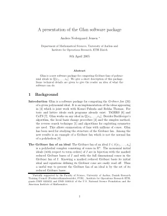
A Presentation of the Gfan Software Anders Nedergaard Jensen Department of Mathematical Sciences, University of Aarhus ICMS, September 2006

Gfan ◮ Gfan is a C++ program for computing Gröbner fans and tropical varieties . ◮ It is a command line tool consisting of many small programs. ◮ It is released under GNU-GPL.

A simple Gröbner fan example Command gfan Input {a-b-ab, aˆ2+ab} Output {{bˆ3-2*bˆ2, a-b+bˆ2} , {bˆ2-b+a, a*b+b-a, aˆ2-b+a} , {b-a-aˆ2, aˆ3+2*aˆ2}} All marked reduced Gröbner bases of the input polynomial ideal I ⊆ Q [ x 1 , . . . , x n ] are computed.

A “definition” of Gröbner fans Buchberger’s algorithm: Input 1 A list of generators of an ideal I ⊆ Q [ x 1 , . . . , x n ] . Input 2 A term order ≺ (represented by a vector in R n ≥ 0 ). Output A reduced Gröbner basis for I w.r.t. ≺ Observe: ◮ Varying Input 2 we get different Gröbner bases. ◮ Two vectors are equivalent if they produce the same Gröbner basis. ◮ The equivalence classes are the maximal cones in the Gröbner fan of I .

Initial forms and initial ideals Let ω ∈ R n . ◮ The weight of a monomial x a := x a 1 n with a ∈ N n is 1 · · · x a n � ω, a � . ◮ The initial form in ω ( f ) of a polynomial f ∈ Q [ x 1 , . . . , x n ] is the sum of terms with maximal weights. Example: in ( 1 , 2 ) ( x 4 1 + 2 x 2 2 + x 1 x 2 + 1 ) = x 4 1 + 2 x 2 2 ◮ The initial ideal of an ideal I ⊆ Q [ x 1 , . . . , x n ] is defined as in ω ( I ) = � in ω ( f ) � f ∈ I

The following things are in bijection ◮ The marked reduced Gröbner bases I ◮ The full-dimensional Gröbner cones ◮ Monomial initial ideals of I The previous example <a^3,b> <a^2,ab,b^2> <a,b^3> From a marked reduced Gröbner basis it is easy to read off the initial ideal and the defining inequalities of the Gröbner cone.

List of Gfan programs gfan gfan_buchberger gfan_doesidealcontain gfan_facets gfan_fvector gfan_groebnercone gfan_homogeneityspace gfan_homogenize gfan_initialforms gfan_interactive gfan_ismarkedgroebnerbasis gfan_leadingterms gfan_markpolynomialset gfan_polynomialsetunion gfan_render gfan_renderstaircase gfan_stats gfan_substitute gfan_tolatex gfan_tropicalbasis gfan_tropicalintersection gfan_tropicalstartingcone gfan_tropicaltraverse gfan_weightvector

Combining Gfan programs on the UNIX shell Commands gfan|gfan_render > output.fig Input {aab-c,bbc-a,cca-b} Output The following picture stored as an X-fig file Do you see the symmetry?

Exploiting symmetry We wish to exploit the A 3 ⊆ S 3 symmetry: Commands gfan --symmetry | gfan_render > output.fig Input {aab-c,bbc-a,cca-b} {(1,2,0)} Output The following picture stored as an X-fig file We enumerate one Gröbner basis from each symmetry class.

The initial ideal definition of the Gröbner fan ◮ Let I ⊆ Q [ x 1 , . . . , x n ] be a homogeneous ideal. ◮ Define an equivalence relation ∼ on R n . u ∼ v ⇔ in u ( I ) = in v ( I ) ◮ The closure of each equivalence class is called a Gröbner cone. ◮ The set of all these cones is a polyhedral complex. ◮ We call this the Gröbner fan of I .

The tropical semi-ring In the tropical semi-ring ( R , ⊕ , ⊙ ) the operations are ⊕ maximum ⊙ addition Two examples: 5 ⊙ ( 3 ⊕ 2 ) = 8 5 ⊙ 3 ⊕ 5 ⊙ 2 = 8 This explains the word “tropical”. ◮ Tropical polynomial functions are piecewise linear. ◮ The tropical semi-ring gives rise to tropical varieties. ◮ We will define them using initial ideals.

Tropical varieties ◮ Let I ⊆ Q [ x 1 , . . . , x n ] be a polynomial ideal. ◮ We define the tropical variety of I : T ( I ) = { v ∈ R n | in v ( I ) is monomial-free } ◮ T ( I ) is a union of Gröbner cones. ◮ We may think of the tropical variety as a polyhedral complex inheriting its structure from the Gröbner fan. ◮ The tropical variety is a subcomplex of the Gröber fan.

Tropical varieties of prime ideals If I ⊆ Q [ x 1 , . . . , x n ] is a prime ideal of dimension d then ◮ the tropical variety of I is pure d-dimensional. ◮ the tropical variety is connected in codimension one. This allows an algorithm to traverse the d-dimensional cones in a breadth-first way.

Representing Gröbner cones ◮ While n-dimensional Gröbner cones are naturally represented by reduced Gröbner bases ... ◮ ...a lower dimensional cone is represented by a pair of reduced Gröbner bases ◮ - one for the ideal and one for the initial ideal.

Finding a single d-dimensional cone in the tropical variety of a prime ideal Command gfan_tropicalstartingcone Input { bf-ah-ce, bg-ai-de, cg-aj-df, ci-bj-dh, fi-ej-gh } Output {f*i-e*j, d*h-c*i, d*f+a*j, d*e+a*i, c*e+a*h} {f*i-g*h-e*j, d*h-c*i+b*j, d*f-c*g+a*j, d*e-b*g+a*i, c*e-b*f+a*h}

Traversing the tropical variety of a prime ideal Command gfan_tropicaltraverse Input {f*i-e*j, d*h-c*i, d*f+a*j, d*e+a*i, c*e+a*h} {f*i-g*h-e*j, d*h-c*i+b*j, d*f-c*g+a*j, d*e-b*g+a*i, c*e-b*f+a*h} Output Rays:{ 0: (-1,0,0,0,0,0,0,0,0,0), ... 9: (0,0,0,0,0,-1,0,0,0,0)} Printing dimension 2 cones: { {0,4}, {4,5}, {1,4}, ... {3,8}} ...

A tropical example ◮ Consider the 10 2x2 minors of a 2x5 matrix � x 11 � x 12 x 13 x 14 x 15 a = x 11 x 22 − x 12 x 21 x 21 x 22 x 23 x 24 x 25 b = . . . ◮ Notice bf − ah − ce = 0, bg − ai − de = 0 ... ◮ These relations generate the Grassmann-Plücker ideal I . ◮ The tropical variety of I is pure of dimension 7. ◮ We can draw it as the Petersen graph.

Applications You can use Gfan ◮ to investigate combinatorial structure. ◮ to search for an initial ideal with a special property. ◮ to compute a universal Gröbner basis. - for toric ideals (integer programming) this will give a test set for all cost vectors at once.

Computational example 1 Let I be the ideal generated by the 3x3 minors of a 4x4 matrix   x 11 x 12 x 13 x 14 x 21 x 22 x 23 x 24     x 31 x 32 x 33 x 34   x 41 x 42 x 43 x 44 in the polynomial ring of 16 variables. The Gröbner fan consists of 163032 full dimensional cones. ◮ Without symmetry: 14 hours ◮ With symmetry: 7 minutes (289 orbits) 7 dimensional lineality space.

Computational example 2 Let I be the ideal generated by the 3x3 minors of a 4x4 matrix  x 11 x 12 x 13 x 14  x 21 x 22 x 23 x 24     x 31 x 32 x 33 x 34   x 41 x 42 x 43 x 44 in the polynomial ring of 16 variables. ◮ The tropical variety is 12 dimensional with a 7 dimensional lineality space. ◮ The F-vector is ( 1 , 50 , 360 , 1128 , 1680 , 936 ) . ◮ Traversing the maximal cones with symmetry takes 2 minutes.

Computational example 3 Consider the 20 3x3 minors of a 3x6 matrix   x 11 x 12 x 13 x 14 x 15 x 16 x 21 x 22 x 23 x 24 x 25 x 26   x 31 x 32 x 33 x 34 x 35 x 36 The relations on these generate the Grassmann-Plücker ideal I . ◮ The tropical variety of I is pure of dimension 10 and has a 6 dimensional lineality space. ◮ The 1035 maximal cones were computed in 3-4 hours (102 orbits).

Algorithms ◮ Collart, Kalkbrener, Mall: “Converting bases with the Gröbner walk” (1997) ◮ Fukuda, Jensen, Thomas: “Computing Gröbner fans” (2005) ◮ Bogart, Jensen, Speyer, Sturmfels, Thomas: “Computing tropical varieties” (2005)

Installation To be installed Gfan needs ◮ gcc ◮ gmp library for exact arithmetic ◮ cddlib for polyhedral computations Works on Linux and MacOS X.

Related software ◮ TiGERS (Huber, Thomas) and CaTS - for toric ideals ◮ TOPCOM (Rambau) - the Gröbner fan refines the secondary fan ◮ SAGE (Stein) - William Stein is working on a new interface. Gfan and many other math programs are now accessible through the World Wide Web. Would be interesting to use a more efficient Buchberger implementation.