A Population Approach to Ubicomp System Design Matthew C. Higgs , - PowerPoint PPT Presentation
A Population Approach to Ubicomp System Design Matthew C. Higgs , Mark Girolami , Matthew Chalmers, Muffy Calder, Alistair Morrison, Oana Andrei, Marek Bell, ScottSherwood, & John Rooksby Center for Computational Statistics and
A Population Approach to Ubicomp System Design Matthew C. Higgs ⋆ , Mark Girolami ⋆ , Matthew Chalmers, Muffy Calder, Alistair Morrison, Oana Andrei, Marek Bell, ScottSherwood, & John Rooksby ⋆ Center for Computational Statistics and Machine Learning Department of Statistical Science University College London
Contents Introduction Project Description Vision and Ambition Statistical Analysis Analysis of User Traces User life-time length Future Work Future Apps Socio-technical Predicted Legacy
Project Topics. People. Contributions. Marek Scott Bell Oana Sherwood Andrei Formal Muffy John Rooksby Modelling Calder Human Computer Alistair Interaction Morrison Matthew Chalmers Computer Formal Information Methods Science Visuals App Development Ubiquitous Computing Computer Statistics Socio Technical Statistical Mark Data Industrial Modelling Logging Girolami Collaboration Matthew Higgs
Project Communication. Marek Scott Bell Oana Sherwood Andrei Muffy John Rooksby Calder Alistair Morrison Matthew Chalmers Mark Girolami Matthew Higgs
Existing Infrastructure Contributions. Formal Modelling Scottish Living Premier PlanIT League App Edinburgh Festival Development Statistical Data Industrial Modelling Logging Collaboration
Existing Infrastructure Contributions. Hungry Yoshi Formal Modelling Post Factory App Development Match FFIT App Tracker Statistical Data Industrial Modelling Logging Collaboration
Existing Infrastructure Contributions. Formal Modelling App Development Statistical Data Industrial SGLog Modelling Logging Collaboration
Existing Infrastructure Work flow. Formal Modelling App Development Statistical Data Industrial Modelling Logging Collaboration
Contents Introduction Project Description Vision and Ambition Statistical Analysis Analysis of User Traces User life-time length Future Work Future Apps Socio-technical Predicted Legacy
Adaptive Design The ideal. • Observe software in the wild. • Initiate a positive change based on observation. The ideal is ambiguous about what is observed , what change is made , and who makes the change .
Software in the Wild The emergence of the “app store” market has enabled researchers to run worldwide ubicomp trials with huge numbers of users.
Software in the Wild Study type. Trial Hungry methodology Yoshi Modularity Post Factory App Development Modularity Match FFIT App Tracker Ubiquity
Software in the Wild Study type. Trial methodology Modularity d a t a d a t a d a t a d a t d a d a a t a t d a a t a d d a a t t a a d d a a t a t a d a d t a a d t a a d t a a d t a a d t a a t a d d a Modularity SGLog a t a d d a a t t a t a d a d a a t d t a a d d a t a a t a d a d a t a d a t a t a d a t a d a a t d a a t d a t a d a a t Data d t a Ubiquity a d a d a t Logging
Data Analysis d a t a d a t a d a t a d a t d a d a a t a t d a a t a d d a a t t a a d d User a a t a t models a d a d t a a d t a a d t a a d t a a d t a a t a d d a Software models SGLog a t a d d a a t t a t a d a d a a t d t a a d d a t a a t a d a d a t a d a t a t a d a t a d a a t d a a t d a t a d a Statistical a t Data d t a a d a d a t Modelling Logging
Vision Summary Trials: • Create socio-technical environments and persuade people to immerse themselves. Statistical: • Infer the structure and dynamics in the use and evolution data of software populations. Ambition: • Develop visualisation tools and formal methods to guide “developers” in their design decisions.
Contents Introduction Project Description Vision and Ambition Statistical Analysis Analysis of User Traces User life-time length Future Work Future Apps Socio-technical Predicted Legacy
Analysis of User Traces Consider a string of symbols a = a 1 a 2 · · · a N . (1) Where each symbol a i takes values in a finite set A . Consider a set of strings A = { a u , u = 1 , . . . , M , | a u | = N ( u ) ∈ N } . (2) Assume A to be a set of user traces, where A represents a set of possible actions.
Analysis of User Traces Given a set of user traces A , we want to: • Characterise the natural behaviours of the population. • Summarise the population based on these behaviours. “Natural behaviours” are frequently occurring patterns of actions. A “summary” of the population is a representation of the population in a low dimensional space spanned by latent behavioural semantics. We use Probabilistic Latent Semantic Analysis .
Analysis of User Traces PLSA consists of: • A directed graph (digraph) G ( A , E ) representing the set of possible action transitions in the app. • A set of K transition matrices { T k , k = 1 , . . . , K } over the (actionable) nodes of the graph. • A mixture weighting θ = ( θ 1 , . . . , θ K ) for each user. We assume each string a is generated by: • Moving from a i to a i + 1 using transition T k with probability θ k . An admixture of (first-order) discrete-time Markov chains.
Simplified Hungry-Yoshi (a) Main-menu screen-shot. (b) Yoshi screen-shot. (c) Plantation screen-shot. Symbol Yoshi Feed Plant Pick Description View a yoshi. Feed a yoshi. View a plant. Pick a fruit. (d) Symbol table and descriptions of corresponding in-app events. Yoshi Plant Plant Yoshi Plant Pick Pick Pick Yoshi Feed Feed Feed Plant Pick · · · (e) An example of a typical user-trace.
Hungry-Yoshi Digraph p 3 | 1 p 1 | 3 Yoshi Plant p 1 | 1 p 3 | 3 p 1 | 4 p 3 | 2 p 2 | 1 p 1 | 2 p 3 | 4 p 4 | 3 p 2 | 3 p 4 | 1 Feed Pick p 2 | 2 p 4 | 4 p 2 | 4 p 4 | 2 Figure : Yoshi , Feed , Plant , Pick enumerated as { 1 , 2 , 3 , 4 } .
Hungry-Yoshi PLSA ( K = 2) Plant Plant Yoshi Yoshi Feed Pick Feed Pick (a) Digraph 1. (b) Digraph 2. 1 Value indexed by u (see legend). θ 1|u θ 2|u 0.5 0 −0.5 −1 20 40 60 80 100 120 User index − ordered by θ 1|u (descending). (c) Population weights.
Successful vs. Unsuccessful Strategies Yoshi Plant Yoshi Plant Feed Pick Feed Pick (d) Successful? (e) Unsuccessful? What is the criteria for success ?
Successful vs. Unsuccessful • User is successful if they complete a number of tasks. • Developer is successful if a number of users complete a number of tasks. θ 1|u 1 log(N(u)/2)/s Value indexed by u (see legend). 0.8 0.6 0.4 0.2 0 20 40 60 80 100 120 User index − ordered by θ 1|u (descending). Figure : Population weights with trace-lengths.
PLSA Summary • Maximum Likelihood PLSA is prone to over-fitting, but do we care. • How will developers use the results. (Personalisation vs fragmentation). • How will formal methods use these results. • How do we choose K . • Extend to MDPs, identify “states” and latent reward mechanisms.
Contents Introduction Project Description Vision and Ambition Statistical Analysis Analysis of User Traces User life-time length Future Work Future Apps Socio-technical Predicted Legacy
User life-time length Log−log PF population data plot. 6 5 4 log N(t) 3 2 1 0 0 1 2 3 4 5 log t Figure : Plot of Post-Factory population data on a log-log scale. N ( t ) denotes number of users who performed at least t actions.
Coin-toss game model • Constant bias (CB). Every player in every round uses the same coin with bias p ∈ [ 0 , 1 ] . • Empirical bias (EB). Every player in each round uses the same coin, but in each round a new coin with bias p t ∈ [ 0 , 1 ] is given to all players. • Functional bias (FB). The bias p t is assumed to have a functional form p t = ( 1 − p 0 )( 1 + e − t /α ) + p 0 , (3) where p 0 ∈ [ 0 , 1 ] is an initial probability, and α > 0 a scale parameter.
Coin-toss game model Plot of model parameters as a function of time. 1 0.95 MLE of p(t). 0.9 0.85 CB−model 0.8 EB−model FB−model 0.75 0 50 100 150 t. Figure : Bias parameters for each CTG model, estimated using the full Post-Factory population data set.
Coin-toss game model CB−model MLE. EB−model MLE. FB−model MLE. 6 6 6 5 5 5 4 4 4 log N(t) log N(t) log N(t) 3 3 3 2 2 2 Data Data Data 1 1 1 Mean path Mean path Mean path 0 0 0 0 1 2 3 4 5 0 1 2 3 4 5 0 1 2 3 4 5 log t log t log t Figure : Mean path plots for each of the CTG models. CB-model EB-model FB-model 2-fold 71.9 ± 17.4 17.5 ± 12.2 14.8 ± 11.6 5-fold 13.1 ± 1.74 4.44 ± 1.57 4.25 ± 1.52 10-fold 4.12 ± 0.48 1.97 ± 0.46 1.93 ± 0.45 Figure : Estimates of MSE using K -fold CV. Mean MSE ± one std, from 10,000 reps.
CTG Summary • The best performer is the FB-model with bias p t = ( 1 − p 0 )( 1 + e − t /α ) + p 0 . (4) • This is a psychometrically motivated choice model . • p 0 can be thought of as a function of the properties of the app at start up. • α can be thought of as a reward rate that determines how “attached” the user becomes with time.
Recommend
More recommend
Explore More Topics
Stay informed with curated content and fresh updates.
