A little stochastic calculus: Hull, ch. 13 & 14. Assume dS S = - PDF document

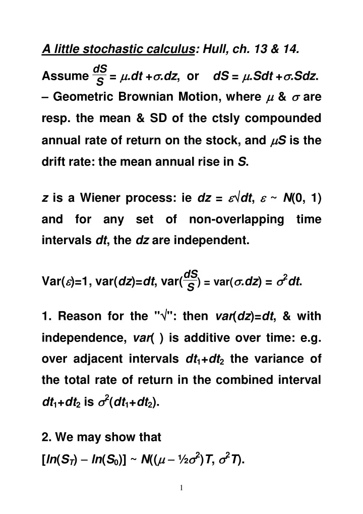
A little stochastic calculus: Hull, ch. 13 & 14. Assume dS S =  .dt +  .dz , or dS =  .Sdt +  .Sdz . – Geometric Brownian Motion, where  &  are resp. the mean & SD of the ctsly compounded annual rate of return on the stock, and  S is the drift rate: the mean annual rise in S . z is a Wiener process: ie dz =  dt ,  ~ N (0, 1) and for any set of non-overlapping time intervals dt , the dz are independent. Var(  )=1, var( dz )= dt , var( dS S ) = var(  .dz ) =  2 dt . 1. Reason for the "  ": then var ( dz )= dt , & with independence, var ( ) is additive over time: e.g. over adjacent intervals dt 1 + dt 2 the variance of the total rate of return in the combined interval dt 1 + dt 2 is  2 ( dt 1 + dt 2 ). 2. We may show that [ ln ( S T )  ln ( S 0 )] ~ N ((   ½  2 ) T ,  2 T ). 1

3. Set up a portfolio in the stock and a call written on it. Both affected by same source of uncertainty: movements in S . In dt , c and S are perfectly correlated, and you can form a riskless hedge. c = c ( S ), so c has the same underlying stochastic process as S . [Technically: use Itô's lemma to get stochastic process for c . Also need this to prove 2.] The value of the portfolio is  =  c + hS d  =  dc + hdS , which turns out not to involve z if the hedge ratio h is appropriately chosen: can eliminate risk  d  = R F  dt  implied 'no arbitrage' price of option.  B&S's partial differential equation for c in terms of S and t , with  and R F as parameters. Doesn't involve  . Solve, s.t. a boundary condition c ( T ) = max ( S T  E , 0)  2

c = SN ( d 1 )  Ee  R F T N ( d 2 ) the B&S equation. The d s are functions of S , T ,  , R F , E , and N ( d ) is the area under the LH tail of the normal curve up to d . 4. Alternatively: at expiry, call is worth either S T  E or 0, and the expected value of this is (where E is the expectation operator): E ( S T  S T  E )  E .prob( S T  E ). Given the distribution of S (2. above), replacing  with R F (for a risk- neutral world), we may evaluate this. In a risk neutral world, all cashflows are discounted at R F , and if we multiply the expression by e  R F T , we get the B&S equation, thus giving us an interpretation of its two parts. 3

Some problems with quantitative finance 1. A common thread: 'normality' as the source of risk. Probably discounts the true P (extreme events) so that options (and other) derivatives are mispriced just when they are needed most. e.g. 5% of the probability lies outside  1.96 S.Ds. 1% outside  2.58 S.Ds. 0.27% outside  3 S.Ds 0.006% outside  4 S.Ds. v. (a) The Fyffes data: 3405 observations Jan. 91-Nov. 05, mean daily change +0.04% with S.D. 2.22%. On 39 days the  change  exceeded 3 S.Ds, compared with an expectation (if normal) of 9 days. Of the 39, 19 days had changes exceeding 4 S.D.s, v. an expectation of 0.2 days. 4

(b) Other evidence of 'fat tails': the 'volatility smile'. See Hull, ch. 19. If the market believes stock returns obey Geometric Brownian Motion (GBM) (i.e. prices lognormal) then European options' ( no div .) prices will be consistent with the B&S model, given the market's average view of volatility,  . Invert this logic: given T , R F and S , apply B&S to the price of an option at any E , and the implied standard deviation ISD that you get should be  , no matter what E you use: Volatility ISD=  S Exercise price E 5

In fact for equity options a plot of ISD v. E frequently looks something like: Far out-of-the-money (FOTM) Volatility puts have a much higher ISD than at-the-money puts. Calls ISD likewise at these low values of E. E fotm put S Exercise price E As put (& call) prices are positively related to  , this suggests that the market is placing a higher value on FOTM puts (& calls at those execrcise prices, because of put-call-parity) than B&S, i.e. the market is not consistent with B&S.  the market puts a higher probability than GBM/lognormal on exercising FOTM puts: it has detected that the lower tail of the distribution is in fact fatter than GBM/lognormal. 6

2. In view of 1., how to model stock prices? Perhaps Merton's 'Jump diffusion process': combines GBM with possibility of discrete jumps, generated by a Poisson process. 3. Pricing of derivatives in general depends on the pricing of a replicating PF: e.g. c = price of a stock/cash combination; futures F likewise. What if the other markets aren't frictionless & liquid? restrictions on short selling? ____ Conclusion: Pricing models & trading strategies based on normality/GBM, in a world of market frictions, can  incorrect action. The underlying 'riskless arbitrage' won't be riskless. Note the implications when B&S is used to compute the 'hedge ratio': e.g. for 'delta hedging'; e.g. for constructing synthetic options from other assets. 7