A case study on using generalized additive models to fit credit - PowerPoint PPT Presentation
A case study on using generalized additive models to fit credit rating scores Marlene Mller, marlene.mueller@itwm.fraunhofer.de This version: July 8, 2009, 14:32 Contents Application: Credit Rating Aim of this Talk Case Study German
A case study on using generalized additive models to fit credit rating scores Marlene Müller, marlene.mueller@itwm.fraunhofer.de This version: July 8, 2009, 14:32
Contents Application: Credit Rating Aim of this Talk Case Study German Credit Data Australian Credit Data French Credit Data UC2005 Credit Data Simulation Study Conclusions Appendix: Further Plots Australian Credit Data French Credit Data UC2005 Credit Data 1
Application: Credit Rating - Basel II: capital requirements of a bank are adapted to the individual credit portfolio - core terms: determine rating score and subsequently default probabilities (PDs) as a function of some explanatory variables - further terms: loss given default, portfolio dependence structure - in practice: often classical logit/probit-type models to estimate linear predictors (scores) and probabilities (PDs) - statistically: 2-group classification problem risk management issues - credit risk is ony one part of a bank’s total risk: � will be aggregated with other risks - credit risk estimation from historical data: � stress-tests to simulate future extreme situations � need to easily adapt the rating system to possible future changes � possible need to extrapolate to segments without observations 2
Application: Credit Rating - Basel II: capital requirements of a bank are adapted to the individual credit portfolio - core terms: determine rating score and subsequently default probabilities (PDs) as a function of some explanatory variables - further terms: loss given default, portfolio dependence structure - in practice: often classical logit/probit-type models to estimate linear predictors (scores) and probabilities (PDs) - statistically: 2-group classification problem risk management issues - credit risk is ony one part of a bank’s total risk: � will be aggregated with other risks - credit risk estimation from historical data: � stress-tests to simulate future extreme situations � need to easily adapt the rating system to possible future changes � possible need to extrapolate to segments without observations 2
(Simplified) Development of Rating Score and Default Probability � raw data: X j measurements of several variables (“risk factors”) � (nonlinear) transformation: X j → e X j = m j ( X j ) � handle outliers, allow for nonlinear dependence on raw risk factors � rating score: S = w 1 e X 1 + . . . + w d e X d � default probability: PD = P ( Y = 1 | X ) = G ( w 1 e X 1 + . . . + w d e X d ) (where G is e.g. the logistic or gaussian cdf � logit or probit) 3
(Simplified) Development of Rating Score and Default Probability � raw data: X j measurements of several variables (“risk factors”) � (nonlinear) transformation: X j → e X j = m j ( X j ) � handle outliers, allow for nonlinear dependence on raw risk factors � rating score: S = w 1 e X 1 + . . . + w d e X d � default probability: PD = P ( Y = 1 | X ) = G ( w 1 e X 1 + . . . + w d e X d ) (where G is e.g. the logistic or gaussian cdf � logit or probit) 3
(Simplified) Development of Rating Score and Default Probability � raw data: X j measurements of several variables (“risk factors”) � (nonlinear) transformation: X j → e X j = m j ( X j ) � handle outliers, allow for nonlinear dependence on raw risk factors � rating score: S = w 1 e X 1 + . . . + w d e X d � default probability: PD = P ( Y = 1 | X ) = G ( w 1 e X 1 + . . . + w d e X d ) (where G is e.g. the logistic or gaussian cdf � logit or probit) 3
(Simplified) Development of Rating Score and Default Probability � raw data: X j measurements of several variables (“risk factors”) � (nonlinear) transformation: X j → e X j = m j ( X j ) � handle outliers, allow for nonlinear dependence on raw risk factors � rating score: S = w 1 e X 1 + . . . + w d e X d � default probability: PD = P ( Y = 1 | X ) = G ( w 1 e X 1 + . . . + w d e X d ) (where G is e.g. the logistic or gaussian cdf � logit or probit) 3
(Simplified) Development of Rating Score and Default Probability � raw data: X j measurements of several variables (“risk factors”) � (nonlinear) transformation: X j → e X j = m j ( X j ) � handle outliers, allow for nonlinear dependence on raw risk factors � rating score: S = w 1 e X 1 + . . . + w d e X d � default probability: PD = P ( Y = 1 | X ) = G ( w 1 e X 1 + . . . + w d e X d ) (where G is e.g. the logistic or gaussian cdf � logit or probit) 3
Aim of this Talk case study on (cross-sectional) rating data - compare different approaches to generalized additive models (GAM) - consider models that allow for additional categorical variables � partial linear terms (combination of GAM/GPLM) � generalized additive models allow for a simultaneous fit of the transformations from the raw data, the linear rating score and the default probabilities 4
Outline of the Study � credit data case study: 4 credit datasets regressors dataset sample defaults continuous discrete categorical German Credit 1000 30.00% 3 – 17 Australian Credit 678 55.90% 3 1 8 French Credit 8178 5.86% 5 3 15 UC2005 Credit 5058 23.92% 12 3 21 - differences between different approaches? - improvement of default predictions? � simulation study: comparison of additive model (AM) and GAM fits - differences between different approaches? - what if regressors are concurve? (nonlinear version of multicollinear) - do sample size and default rate matter? 5
Generalized Additive Model � logit/probit are special cases of the generalized linear model (GLM) “ ” X ⊤ β E ( Y | X ) = G � “classic” generalized additive model 8 9 < p = X E ( Y | X ) = G : c + m j ( X j ) m j nonparametric ; j = 1 � generalized additive partial linear model (semiparametric GAM) 8 9 < = p X : c + X ⊤ E ( Y | X 1 , X 2 ) = G 1 β + m j ( X 2 j ) m j nonparametric ; j = 1 linear part - allows for known transformation functions - allows to add / control for categorical regressors 6
Generalized Additive Model � logit/probit are special cases of the generalized linear model (GLM) “ ” X ⊤ β E ( Y | X ) = G � “classic” generalized additive model 8 9 < p = X E ( Y | X ) = G : c + m j ( X j ) m j nonparametric ; j = 1 � generalized additive partial linear model (semiparametric GAM) 8 9 < = p X : c + X ⊤ E ( Y | X 1 , X 2 ) = G 1 β + m j ( X 2 j ) m j nonparametric ; j = 1 linear part - allows for known transformation functions - allows to add / control for categorical regressors 6
Generalized Additive Model � logit/probit are special cases of the generalized linear model (GLM) “ ” X ⊤ β E ( Y | X ) = G � “classic” generalized additive model 8 9 < p = X E ( Y | X ) = G : c + m j ( X j ) m j nonparametric ; j = 1 � generalized additive partial linear model (semiparametric GAM) 8 9 < = p X : c + X ⊤ E ( Y | X 1 , X 2 ) = G 1 β + m j ( X 2 j ) m j nonparametric ; j = 1 linear part - allows for known transformation functions - allows to add / control for categorical regressors 6
R “Standard” Tools two main approaches for GAM in - gam::gam � backfitting with local scoring (Hastie and Tibshirani; 1990) - mgcv::gam � penalized regression splines (Wood; 2006) � compare these procedures under the default settings of gam::gam and mgcv::gam competing estimators: - logit binary GLM with G ( u ) = 1 / { 1 + exp ( − u ) } (logistic cdf as link) - logit2 , logit3 binary GLM with 2nd / 3rd order polynomial terms for the continuous regressors - logitc binary GLM with continuous regressors categorized (4–5 levels) - gam binary GAM using gam::gam with s () terms for continuous - mgcv binary GAM using mgcv::gam 7
German Credit Data � from http://www.stat.uni-muenchen.de/service/datenarchiv/kredit/kredit_e.html regressors dataset name sample defaults continuous discrete categorical German 1000 30.00% 3 – 17 � 3 continuous regressors: age, amount, duration (time to maturity) � use 10 CV subsamples for validation � stratified data (true default rate ≈ 5%) � important findings: - some observation(s) that seem to confuse mgcv::gam in one CV subsample ( → see following slides) - however, mgcv::gam seems to improve deviance and discriminatory power w.r.t. gam::gam - estimation times of mgcv::gam are between 4 to 7 times higher than for gam::gam (not more than around a second, though) - if we only use the continuous regressors: both GAM estimators are comparable to logit cubic additive functions 8
German Credit Data � from http://www.stat.uni-muenchen.de/service/datenarchiv/kredit/kredit_e.html regressors dataset name sample defaults continuous discrete categorical German 1000 30.00% 3 – 17 � 3 continuous regressors: age, amount, duration (time to maturity) � use 10 CV subsamples for validation � stratified data (true default rate ≈ 5%) � important findings: - some observation(s) that seem to confuse mgcv::gam in one CV subsample ( → see following slides) - however, mgcv::gam seems to improve deviance and discriminatory power w.r.t. gam::gam - estimation times of mgcv::gam are between 4 to 7 times higher than for gam::gam (not more than around a second, though) - if we only use the continuous regressors: both GAM estimators are comparable to logit cubic additive functions 8
Recommend
More recommend
Explore More Topics
Stay informed with curated content and fresh updates.
