91.304 Foundations of (Th (Theoretical) Computer Science ti l) C - PowerPoint PPT Presentation
91.304 Foundations of (Th (Theoretical) Computer Science ti l) C t S i Chapter 3 Lecture Notes (Section 3.2: Variants of Turing Machines) David Martin dm@cs.uml.edu With some modifications by Prof. Karen Daniels, Fall 2012 This work is
91.304 Foundations of (Th (Theoretical) Computer Science ti l) C t S i Chapter 3 Lecture Notes (Section 3.2: Variants of Turing Machines) David Martin dm@cs.uml.edu With some modifications by Prof. Karen Daniels, Fall 2012 This work is licensed under the Creative Commons Attribution-ShareAlike License. To view a copy of this license, visit http: / / creativecommons.org/ licenses/ by- sa/ 2.0/ or send a letter to Creative Commons, 559 Nathan Abbott Way, Stanford, California 94305, USA. 1
Variants of Turing Machines � R b � Robustness : Invariance under certain In a iance nde ce tain t changes � Wh t ki d f h � What kinds of changes? ? � Stay put! � Multiple tapes M lti l t � Nondeterminism � E � Enumerators t � (Abbreviate Turing Machine by TM.) 2
Stay Put! � Transition function of the form: � Transition function of the form: δ δ × Γ Γ → → × Γ Γ × : : Q Q Q Q { { L, L, R, R, S S } } � Does this really provide additional computational power? � No! Can convert TM with “stay put” feature to one without it How? feature to one without it. How? � Theme: Show 2 models are equivalent by showing they can simulate each other . 3
Multi-Tape Turing Machines � Ordinary TM with several tapes. � Ordinary TM with several tapes � Each tape has its own head for reading and writing. � Initially the input is on tape 1, with the other tapes bl blank. k � Transition function of the form: δ × Γ → × Γ × k k k : Q Q { L, R, S } � ( k = number of tapes) δ = K K K ( q , a , , a ) ( q , b , , b , L, R, L ) i 1 k j 1 k � When TM is in state q i and heads 1 through k are reading symbols a 1 through a k , TM goes to state q j , writes symbols b 1 through b k , and moves associated tes sy bo s b 1 t oug b k , a d o es assoc ated tape heads L, R, or S. Note: k tapes (each with own alphabet) but only 1 common set of states! 4 Source: Sipser textbook
Multi-Tape Turing Machines � Multi tape Turing machines are of equal � Multi-tape Turing machines are of equal computational power with ordinary Turing machines! � Corollary 3.15: A language is Turing- recognizable if and only if some multi-tape Turing machine recognizes it. Turing machine recognizes it � One direction is easy (how?) � The other direction takes more thought… � Theorem 3.13: Every multi-tape Turing machine has an equivalent single-tape Turing machine. � Proof idea: see next slide… 5 Source: Sipser textbook
Theorem 3.13: Simulating Multi-Tape g p Turing Machine with Single Tape � Proof Ideas: � Proof Ideas: � Simulate k -tape TM M ’s operation using single-tape TM S . � Create “virtual” tapes and heads. � # is a delimiter separating contents of one tape from another tape’s contents. � “Dotted” symbols represent head positions � add to tape alphabets. k = 3 tapes 6 Source: Sipser textbook
Theorem 3.13: Simulating Multi-Tape g p Turing Machine with Single Tape (cont.) w = = L � � w w w w w Processing input: Processing input: 1 n � Format S ’s tape (different blank symbol v for presentation purposes): ∨ ∨ & & & L L # w w w # # # # 1 2 n � Simulate single move: � Scan rightwards to find symbols under virtual heads. � Update tapes according to M ’s transition function. � Caveat: hitting right end (# ) of a virtual tape: � rightward shift of S ’s tape by 1 unit and insert blank, then continue simulation Why? 7 Source: Sipser textbook
Nondeterministic Turing Machines δ δ × × Γ Γ → → × × Γ Γ × × P P � � : : Q Q ( ( Q Q { { L, L R R }) }) Transition function: Transition function: � Computation is a tree whose branches correspond to different possibilities. Example: board work � � If some branch leads to an accept state, machine accepts. If some branch leads to an accept state machine accepts � Nondeterminism does not affect power of Turing machine! � Theorem 3 .1 6 : Every nondeterministic Turing machine ( N ) has an equivalent deterministic Turing machine ( D ). h i l t d t i i ti T i hi ( D ) � Proof Idea: Simulate, simulate! never changed copy of N ’s tape on some branch of nondeterministic computation keeps track of D ’s location in N ’s keeps track of D s location in N s nondeterministic computation tree 8 Source: Sipser textbook
Theorem 3.16 Proof (cont.) � Proof Idea (continued) � View N ’s computation on input as a tree. � Each node is a configuration. � Search for an accepting configuration. � Important caveat: searching order matters � DFS vs. BFS (which is better and why? ) � � E Encoding location on address tape: di l ti dd t � Assume fan-out is at most b (what does this correspond to? ) Each node has address that is a string over alphabet: Σ b = { 1… � b } never changed copy of N ’s tape on some branch of nondeterministic computation keeps track of D ’s location in N ’s nondeterministic computation tree 9 Source: Sipser textbook
Theorem 3.16 Proof (cont.) � Operation of deterministic TM D : 1. Put input w onto tape 1. Tapes 2 and 3 are empty. 2. Copy tape 1 to tape 2. 3. Use tape 2 to simulate N with input w on one branch. 1. Before each step of N , consult tape 3 (why?) 4. Replace string on tape 3 with lexicographically next string. Simulate next branch of N ’ s computation by going back to step 2. never changed copy of N ’s tape on some branch of nondeterministic computation keeps track of D ’s location in N ’s keeps track of D s location in N s nondeterministic computation tree 10 Source: Sipser textbook
Consequences of Theorem 3.16 � Corollary 3.18: � Corollary 3 18: � A language is Turing-recognizable if and only if some nondeterministic Turing machine recognizes it recognizes it. � Proof Idea: � One direction is easy (how?) � � Other direction comes from Theorem 3 16 Other direction comes from Theorem 3.16. � Corollary 3.19: � A language is decidable if and only if some nondeterministic Turing machine decides it. � Proof Idea: � Modify proof of Theorem 3.16 (how?) 11
Another model � Definition An enum erator E is a 2-tape TM with a special (2 nd tape is for printing) state named q p ("print") � The language generated by E is (tape 1) (tape 2) L(E) = { x ∈ Σ * | (q 0 t , q 0 t ) ` * ( u q p v, x q p z ) for some u, v, z ∈ Γ * } � � Here the instantaneous description is split into two parts Here the instantaneous description is split into two parts (tape1, tape2) � So this says that "x appears to the left of the tape 2 head when E enters the q p state" � � Note that E always starts with a blank tape and potentially Note that E always starts with a blank tape and potentially runs forever � Basically, E generates the language consisting of all the strings it decides to print � And it doesn't matter what's on tape 1 when E prints 12 Source: Sipser textbook
Theorem 3.21 L ∈ Σ 1 ⇔ L= L(E) for some enumerator E (in L ∈ Σ 1 ⇔ L L(E) for some enumerator E (in other words, enumerators are equivalent to TMs) (Recall Σ 1 is set of Turing-recognizable languages.) Proof First we show that L= L(E) ⇒ L ∈ Σ 1 So Proof First we show that L= L(E) ⇒ L ∈ Σ 1 . So assume that L= L(E); we need to produce a TM M such that L= L(M). We define M as a 3-tape TM that works like this: TM that works like this: 1. input w (on tape # 1) 2. run E on M's tapes # 2 and # 3 p 3. whenever E prints out a string x, compare x to w; if they are equal, then accept else goto 2 and continue running E g g So, M accepts input strings (via input w) that appear on E’s list. 13
Theorem 3.21 continued Now we show that L ∈ Σ 1 ⇒ L= L(E) for some Now we show that L ∈ Σ 1 ⇒ L= L(E) for some enumerator E. So assume that L= L(M) for some TM M; we need to produce an ; p enumerator E such that L= L(E). First let s 1 , s 2 , L be the lexicographical enumeration of Σ * (strings over M’s alphabet). E behaves as follows: E b h f ll 1. for i: = 1 to ∞ 2 2. run M on input s i run M on input s i 3. if M accepts s i then print string s i (else continue with next i) DOES NOT W ORK!! DOES NOT W ORK!! W HY?? 14
Theorem 3.21 continued Now we show that L ∈ Σ 1 ⇒ L= L(E) for some enumerator Now we show that L ∈ Σ 1 ⇒ L L(E) for some enumerator E. So assume that L= L(M) for some TM M; we need to produce an enumerator E such that L= L(E). First let be the lexicographical enumeration of Σ * E s 1 , s 2 , L be the lexicographical enumeration of Σ . E s s behaves as follows: 1 1. f for t: = 1 to ∞ t 1 t / * t = time to allow * / 2. for j: = 1 to t / * continue resumes here * / 3. compute the instantaneous description uqv in M such that q 0 s j ` t uqv. (If M halts before t ` t h th t (If M h lt b f t steps, then continue ) exactly t steps of the ` relation 4. if q = q acc then print string s j (else continue ) (else continue ) 15
Recommend
More recommend
Explore More Topics
Stay informed with curated content and fresh updates.
