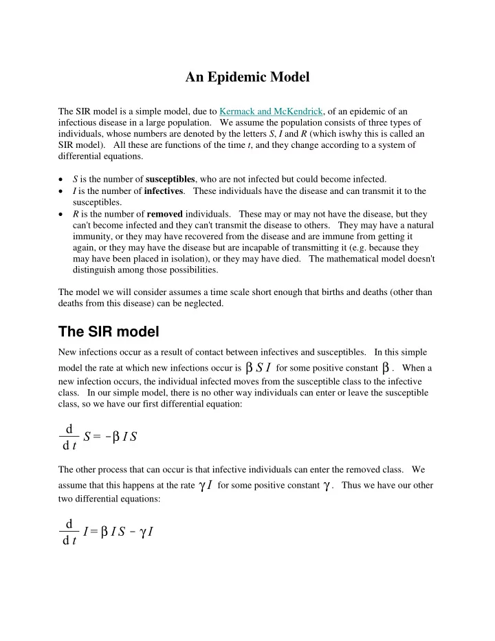

An Epidemic Model The SIR model is a simple model, due to Kermack and McKendrick, of an epidemic of an infectious disease in a large population. We assume the population consists of three types of individuals, whose numbers are denoted by the letters S , I and R (which iswhy this is called an SIR model). All these are functions of the time t , and they change according to a system of differential equations. S is the number of susceptibles , who are not infected but could become infected. I is the number of infectives . These individuals have the disease and can transmit it to the susceptibles. R is the number of removed individuals. These may or may not have the disease, but they can't become infected and they can't transmit the disease to others. They may have a natural immunity, or they may have recovered from the disease and are immune from getting it again, or they may have the disease but are incapable of transmitting it (e.g. because they may have been placed in isolation), or they may have died. The mathematical model doesn't distinguish among those possibilities. The model we will consider assumes a time scale short enough that births and deaths (other than deaths from this disease) can be neglected. The SIR model New infections occur as a result of contact between infectives and susceptibles. In this simple model the rate at which new infections occur is for some positive constant . When a new infection occurs, the individual infected moves from the susceptible class to the infective class. In our simple model, there is no other way individuals can enter or leave the susceptible class, so we have our first differential equation: The other process that can occur is that infective individuals can enter the removed class. We assume that this happens at the rate for some positive constant . Thus we have our other two differential equations:
Some things to notice: The total population is constant because For convenience, I'll usually choose the unit of population so that the total population is 1. If , i.e. there are no infectives, the right sides of all three equations are 0, so nothing changes. To make matters interesting, we must start with some infectives. Here are some of the questions we would like to answer: Suppose we start with a population of almost all susceptibles plus a small number of infectives. Will the number of infectives increase substantially, producing an epidemic, or will the disease fizzle out? Assuming there is an epidemic, how will it end? Will there still be any susceptibles left when it is over? How long will the epidemic last? Before doing any analysis, let's try some numerical simulations. You can choose arbitrary values for the parameters β and , the initial values of S , I and R at time 0, and the end time for the simulation, press the Go button, and see the results. The plot will show in green, in red and in black. You might try some cases with and some with : we'll see in the next section why this makes a difference. 8.0 4.3
.99 0.01 .0 end time 2.65198
S 2.65198 2.65198 = 0.249766309 = 0.00999987565 2.65198 = 0.740233815 S and I Our SIR model is a system of three differential equations, with three unknown functions. Perhaps you have only studied single differential equations, with one unknown function. Don't let that bother you! Fortunately, there is a simple trick that will "reduce" this problem to a single differential equation. The idea is to consider I as a function of S . According to the chain rule Since the right side depends only on S and not on I , to solve this differential equation all we have to do is integrate: where C is an arbitrary constant. The value of C can be found by plugging in the initial condition: . Here you can choose values for β and and plot I as a function of S for various choices of . 5.0 3.6
Notice that because the formulas differ only by the additive constant C , these curves are all vertical translates of each other. Mathematically the curves extend to negative values of I as well as positive, but of course that doesn't make sense for populations, so I cut them off at . The line really consists of equilibrium points: if nothing will happen in our model. If you start out at a point on one of these curves with , as time goes on you travel along the curve to the left (because ), eventually approaching at some positive value of . This must happen since on any of these curves, as .So the answer to question (2) is that the epidemic will end as with approaching some positive value: yes, there must always be some susceptibles left over. To see how many will be left over, we must find the value of that satisfies the
equation . This equation can't be solved using elementary methods because of the presence of both S and , but it can be solved using numerical methods or with a special function called the Lambert W function: the solution is . The Go button below will find the result, given values of β , , and . It should agree fairly closely with the simulation (not exactly, because of roundoff error). 8.0 8.3 .99 0.01 0.8929091912
For the answer to (1), note that if , which happens if . If that's true at the start, it remains true because S is decreasing. If I started out small, it just keeps getting smaller, and the disease fizzles out. On the other hand, if , so the epidemic "takes off": the number of infectives increases until S has decreased to the value . We can say that what determines whether the epidemic "takes off'' is which occurs faster: new infections (at the rate ) or removal of infectives (at the rate ). If you want to prevent epidemics, you need to ensure that . For example, you might try to reduce S by immunizing some of the population; you don't have to immunize . Or you might try to reduce β by encouraging people to everybody, just enough so wash their hands more. How long? Now for question (3), we must go back to a differential equation involvingtime. Plugging in the formula for I as a function of S into the differential equation for , we get To solve this differential equation using separation of variables, write Unfortunately we don't know an antiderivative for the left side: there probably isn't a formula for it. But numerical methods can be used.
Let's say we start with (some small positive number) and where . Thus . The epidemic will "take off" and then eventually die out. However, we never quite get to , just approach it in the limit as . So what can I take as the "end" of the epidemic? Let's say it's over when comes back to the value . This will happen when , where We can solve this for , again using the Lambert W function. Once we have that value, we use it as the upper endpoint in the integral to find the duration T of the epidemic. The Go button below will perform these calculations. 8.0 2.3 .99 0.01 3.075850568
The zombie apocalypse Many variations on this basic SIR model have been considered. One interesting case that was published in 2009 by Philip Munz, Ioan Hudea, Joe Imad and Robert J. Smith is a model of a zombie apocalypse. In its simplest form the system of differential equations is Here S are susceptibles (normal live humans), Z are zombies and R are dead (but not permanently so!). Encounters between zombies and live humans can result in the human becoming a zombie (hence the terms in and in ) or the zombie becoming dead (hence the and ). The dead sometimes spontaneously turn into zombies (hence the and terms). The result is unfortunate: unless both S and R start out at 0, the whole population must turn into zombies in the limit as . Here is a numerical simulation of the system. 1.0 4.0 0.2
.99 0.01 .00 end time 100
S 100 100 = 0.993411341 = 4.96907619 10-11 100 = 0.00658865861
Recommend
More recommend