5.3 Nonlinear models (with 4.10 material too) a lesson for MATH - PowerPoint PPT Presentation

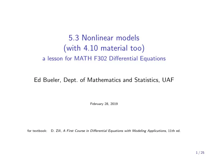
5.3 Nonlinear models (with 4.10 material too) a lesson for MATH F302 Differential Equations Ed Bueler, Dept. of Mathematics and Statistics, UAF February 28, 2019 for textbook: D. Zill, A First Course in Differential Equations with Modeling Applications , 11th ed. 1 / 25

outline examples of nonlinear 2nd-order differential equations (DEs): • pendulum ( § 5.3) • using a numerical solver in Matlab / Octave (see § 4.10) • hard and soft springs ( § 5.3) • non-constant gravity: from earth to high orbit ( § 5.3) • dependent variable missing ( § 4.10) 2 / 25

nonlinear pendulum • suppose a pendulum oscillates (swings back and forth) without resistance • if you believe my § 5.1 slides then it must be modeled by a 2nd-order linear DE ◦ this is true for small oscillations ◦ for bigger oscillations (more than 20 ◦ ?) a nonlinear model is more accurate • the DE which comes from the diagram: m ℓ d 2 θ dt 2 = − mg sin θ ◦ you are not responsible for the derivation ◦ . . . but s = ℓθ is arclength, so ℓ d 2 θ dt 2 is acceleration, and only the tangential force is relevant 3 / 25

linear small angle model d 2 θ dt 2 + g • divide by m ℓ and move term: ℓ sin θ = 0 � g d 2 θ dt 2 + ω 2 sin θ = 0 • if ω = ℓ then for any angle • recall sin θ ≈ θ for small θ because sin z = z − z 3 3! + z 5 5! − . . . • a small angle model : d 2 θ dt 2 + ω 2 θ = 0 ◦ solution: θ ( t ) = c 1 cos( ω t ) + c 2 sin( ω t ) 4 / 25

nonlinear versus linearized pendulum nonlinear: any angles linearized: small angles θ ′′ + ω 2 sin θ = 0 θ ′′ + ω 2 θ = 0 solution? θ ( t ) = c 1 cos( ω t ) + c 2 sin( ω t ) � • ω = g /ℓ in both DEs • we don’t know how to solve a nonlinear DE like a pendulum ◦ the term “sin θ ” is not linear: sin( a + b ) � = sin( a ) + sin( b ) 5 / 25

what to do about a nonlinear DE? • for example, the pendulum DE: θ ′′ + ω 2 sin θ = 0 • read section 4.10! − gives advice, not a method ← • what to do about a nonlinear equation like this? ◦ θ = e rt is not a solution for any r (real or complex) ◦ using the concept of energy makes progress (Mini-Project 3) . . . but we get a hard-to-solve 1st-order equation ◦ using infinite series can make progress too (Chapter 6) . . . but basically only gives approximations • numerical approximations can be used for an IVP! ◦ Euler’s method? . . . inefficient but would work ◦ but the equation is second order . . . how does Euler even work? ◦ next: using an efficient “black box” solver in Matlab / Octave 6 / 25

systems of 1st-order ODEs idea: 2nd-order ODE is equivalent to a system of 1st-order ODEs Example. convert into a 1st-order system: √ x ′′ + 5( x ′ ) 2 + sin x ∗ = t Solution. Second derivative x ′′ ( t ) is merely the derivative of x ′ ( t ). So give x ′ a name: y = x ′ . Now rewrite ∗ using y : √ y ′ + 5 y 2 + sin x = t . Rearrange above two equations to a system: x ′ = y √ y ′ = − 5 y 2 − sin x + t Summary: Ignore the complexity of ∗ . Don’t solve anything, just restate the problem. 7 / 25

pendulum as a 1st-order system exercise. convert into a 1st-order system with initial conditions: θ ′′ + ω 2 sin θ = 0 , θ ′ (0) = B θ (0) = A , solution. z ′ 1 = z 2 z 1 (0) = A 2 = − ω 2 sin( z 1 ) , z ′ z 2 (0) = B 8 / 25

using black-box solver ode45 • before we get to numerical solutions of systems, let’s do a single 1st-order IVP • you can use Octave Online to do the following • or use Matlab or Octave on your own computer example. solve for y ( t ) on 0 ≤ t ≤ 2, and estimate y (2): y ′ = − 3 y + e − t , y (0) = 1 solution. the DE is y ′ = f ( t , y ) so 1 >> f = @(t,y) -3*y + exp(-t); >> [tt,yy] = ode45(f,[0,2],1); 0.8 >> plot(tt,yy) 0.6 >> yy(end) 0.4 ans = 0.068908 0.2 0 0 0.5 1 1.5 2 9 / 25

in Octave Online 10 / 25

only 12 steps, but accurate • the ode45 black-box is quite accurate • exercise. solve by hand for the exact value y (2): y ′ = − 3 y + e − t , y (0) = 1 solution. • compare to y(end)=y(13) on previous slides: >> 0.5*(exp(-2)+exp(-6)) ans = 0.068907 • Euler would need 10 5 or 10 6 steps for this accuracy 11 / 25

calling ode45 • from the Matlab documentation page on ode45 : [t,y] = ode45(odefun,tspan,y0) , where tspan = [t0 tf] , integrates the system of differ- ential equations y ′ = f ( t , y ) from t0 to tf with initial conditions y0 . Each row in the solution array y corre- sponds to a value returned in column vector t . • see the Matlab page for examples of functions f ( t , y ) for the odefun argument • note further fine print about the tspan argument: ◦ If tspan has two elements [t0 tf] then the solver returns the solution evaluated at internal integration steps in the interval. ◦ If tspan has more than two elements [t0,t1,t2,...,tf] then the solver returns the solution evaluated at the given points. 12 / 25

ode45 for pendulum √ example . let ω = 7. solve for θ ( t ) on the interval t ∈ [0 , 20]: θ ′′ + ω 2 sin θ = 0 , θ ′ (0) = 0 θ (0) = 3 , solution. z 1 = θ and ω 2 = 7 so z ′ 1 = z 2 z 1 (0) = 3 z ′ 2 = − 7 sin( z 1 ) z 2 (0) = 0 This is z ′ = f ( t , z ) so: 6 θ (t) d θ /dt >> f = @(t,z) [z(2); -7*sin(z(1))]; 4 >> [tt,zz] = ode45(f,[0,20],[3;0]); 2 >> plot(tt,zz) 0 >> xlabel t >> legend(’\theta(t)’,’d\theta/dt’) -2 -4 -6 0 5 10 15 20 t 13 / 25

pendulum: better and movier • the solution is more accurate than it looks! • for better appearance, generate more points (left fig.): >> [tt,zz] = ode45(f,[0:.01:20],[3;0]); >> plot(tt,zz), xlabel t • one can also make a movie ◦ see pendmovie.m at Codes at bueler.github.io/math302 ◦ right fig. is a frame 6 θ (t) d θ /dt 4 2 0 -2 -4 -6 0 5 10 15 20 t 14 / 25

back to linear mass-spring example . solve for x ( t ) on the interval t ∈ [0 , 20]: x ′′ + 7 x = 0 , x (0) = 3 , x ′ (0) = 0 exact solution. 4 nonlinear θ (t) √ linear x(t) x ( t ) = 3 cos( 7 t ) 2 0 -2 -4 continuing previous code: 0 5 10 15 20 t >> plot(tt,zz(:,1),’b’,tt,3*cos(sqrt(7)*tt),’g’) >> xlabel t >> legend(’nonlinear \theta(t)’,’linear x(t)’) 15 / 25

linear mass-spring: exact vs. numerical • this is a good case on which to check accuracy • example . find x (20): x ′′ + 7 x = 0 , x ′ (0) = 0 x (0) = 3 , √ exact solution. x (20) = 3 cos( 7(20)) = − 2 . 6441 numerical solution. z 1 = x and z 2 = x ′ so z ′ 1 = z 2 z 1 (0) = 3 z ′ 2 = − 7 z 1 z 2 (0) = 0 >> fl = @(t,z) [z(2); -7*z(1)]; >> [ttl,zzl] = ode45(fl,[0:.01:20],[3;0]); >> zzl(end,1) ans = -2.6492 • what about plots of the exact and numerical solutions? √ ◦ you won’t see difference: x ( t ) = 3 cos( 7 t ) versus zzl(:,1) 16 / 25

nonlinear springs • springs are usually well-modeled by Hooke’s law F ( x ) = − kx for small displacements x from the equilibrium position • . . . but when they are over-extended, or closed coil, etc. then they need different models mx ′′ = F ( x ) F(x) F(x) F(x) F(x) x x x x linear hard soft closed 17 / 25

exercise #9: (numerical) nonlinear spring • so F ( x ) = − x − x 3 is a hard spring model • suppose we also have damping (thus x ( t ) → 0 as t → ∞ ) exercise #9 in § 5.3 : numerically solve d 2 x dt 2 + dx dt + x + x 3 = 0 , x (0) = − 3 , x ′ (0) = 8 solution : write as system using x = z 1 , x ′ = z 2 : z ′ 1 = z 2 z 1 (0) = − 3 2 = − z 2 − z 1 − z 3 z ′ z 2 (0) = 8 1 10 x(t) dx/dt and use ode45 : 5 >> f = @(t,z) [z(2); -z(2)-z(1)-z(1)^3]; >> [tt,zz] = ode45(f,[0:.01:5],[-3;8]); 0 >> plot(tt,zz), xlabel t, grid on >> legend(’x(t)’,’dx/dt’) -5 -10 0 1 2 3 4 5 t 18 / 25

bullet to geosynchronous orbit example . We want to use a bullet weighting 100 grams to destroy a satellite in geosynchronous (geostationary) orbit, approximately 36 , 000 km. What velocity is needed if we ignore air drag? solution . Constant gravity g will not do. The gravity decreases as the bullet rises. From § 5.3 we read Newton’s law of gravitation: my ′′ = − k Mm where m =(bullet mass), M =(earth mass) y 2 After simplification (see text), and with initial conditions, this is y ′′ = − g R 2 y ′ (0) = V y 2 , y (0) = R , We take R = 6 . 4 × 10 6 m =(radius of earth) and g = 9 . 8. ( Note bullet mass does not matter. Earth’s mass is built into g. ) Question: Find V so that the maximum of y ( t ) is 3 . 6 × 10 7 m. 19 / 25

bullet to geosynchronous orbit 2 question: Find V so max y ( t ) = 3 . 6 × 10 7 , given y ′′ = − g R 2 y 2 , y (0) = R , y ′ (0) = V and R = 6 . 4 × 10 6 m =(radius of earth) and g = 9 . 8 solution?: as system with y = z 1 , y ′ = z 2 and C = gR 2 : z ′ 1 = z 2 z 1 (0) = R 2 = − Cz − 2 z ′ z 2 (0) = V 1 >> g = 9.8; R = 6.4e6; C = g*R^2; 8e+06 >> f = @(t,z) [z(2); -C/z(1)^2]; >> V = 5000; 7.5e+06 >> [tt,zz] = ode45(f,[0,1000],[R;V]); >> plot(tt,zz(:,1)) 7e+06 y >> xlabel t, ylabel y >> max(zz(:,1)) 6.5e+06 ans = 7.9924e+06 6e+06 0 200 400 600 800 1000 t 20 / 25