4.1 Online Convex Optimization Definition 4.1.1 In Euclidian space, - PDF document

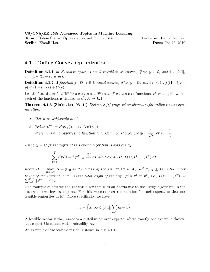
CS/CNS/EE 253: Advanced Topics in Machine Learning Topic: Online Convex Optimization and Online SVM Lecturer: Daniel Golovin Scribe: Xiaodi Hou Date: Jan 13, 2010 4.1 Online Convex Optimization Definition 4.1.1 In Euclidian space, a set C is said to be convex , if ∀ x, y ∈ C , and t ∈ [0 , 1] , z = (1 − t ) x + ty is in C . Definition 4.1.2 A function f : D → R is called convex , if ∀ x, y ∈ D , and t ∈ [0 , 1] , f ((1 − t ) x + y ) ≤ (1 − t ) f ( x ) + tf ( y ) . Let the feasible set X ⊆ R n be a convex set. We have T convex cost functions: c 1 , c 2 , . . . , c T , where each of the functions is defined as c i : X → [0 , 1]. Theorem 4.1.3 (Zinkevich ’03 [1]) Zinkevich [1] proposed an algorithm for online convex opti- mization: 1. Choose x 1 arbitrarily in X 2. Update x t +1 = Proj X x t − η t · ∇ c t ( x t ) � � where η t is a non-increasing function of t . Common choices are η t = 1 t , or η t = 1 √ t . √ Using η t = 1 / t the regret of this online algorithm is bounded by: T √ T + G 2 √ √ c t ( x t ) − c t ( z t ) ≤ D 2 T + 2 D · L ( z 1 , z 2 , . . . , z T ) � T, 2 t =1 x , y ∈X � x − y � 2 is the radius of the set; ∀ t, ∀ x ∈ X , �∇ c t ( x ) � 2 ≤ G is the upper where D = max bound of the gradient, and L is the total length of the drift, from z 1 to z T , i.e., L ( z 1 , . . . , z T ) := i =1 � z i +1 − z i � 2 . � T − 1 One example of how we can use this algorithm is as an alternative to the Hedge algorithm, in the case where we have n experts. For this, we construct a dimension for each expert, so that our feasible region lies in R n . More specifically, we have: n � � � X = x : x i ∈ [0 , 1]; x i = 1 . i =1 A feasible vector x then encodes a distribution over experts, where exactly one expert is chosen, and expert i is chosen with probability x i . An example of the feasible region is shown in Fig. 4.1.1. 1

expert 2 1 x 2 x 1 0 1 expert 1 Figure 4.1.1: An example of the feasible region X in 2D space. The projection operation can be very complex for an arbitrary convex set X . Ideally we want to find the projection: Proj( y ) = argmin � y − x � 2 . (4.1.1) x ∈X 4.2 Support Vector Machine In this section, we will switch some of the previous notations. The data points are denoted as x 1 , x 2 , . . . , x T ∈ R n ; the labels y i are binary variables: y 1 , y 2 , . . . , y T ; y i ∈ {− 1 , 1 } . A linear clas- sifier can be considered as a hyperplane with normal vector w ∈ R n and offset b . The classification of x i is determined by the hyperplane: y i = sign( w · x i + b ) . ˜ (4.2.2) 4.2.1 Eliminating b by augmenting one dimension Eq. 4.2.2 can be expressed in a simpler way, by augmenting x and w . Let x + = [ x 1 , x 2 , . . . , x n , 1] ∈ R n +1 , and w + = [ w 1 , w 2 , . . . , w n , b ], therefore: y = sign( w · x + b ) = sign( w + · x + ) . ˜ For efficiency, we substitute x and w with the augmented vectors x + and w + . 4.2.2 Hinge loss The objective of a linear classifier is to find the hyperplane that “optimally” separates the positive samples from negative ones. In SVM, such optimality is defined as maximizing the margins, or minimizing the hinge loss. T w ⋆ = argmin � hinge( x t , y t , w ) , s.t. � w � 2 ≤ λ. (4.2.3) w t +1 where the hinge function is defined as: � � hinge( x , y, w ) ≡ max 0 , 1 − y ( x · w ) (4.2.4) 2

The hinge function is the least convex upper-bound of the 0 − 1 loss function. Both functions are drawn in Fig. 4.2.2. 1 1 0 1 0 1 A) 0-1 loss func�on B) Hinge loss func�on Figure 4.2.2: Figure A: the 0-1 loss function. Figure B: the hinge loss function. 4.2.3 Online SVM Given the data points x 1 , x 2 , . . . x T ∈ R n +1 , and the corresponding labels y 1 , y 2 , . . . , y T ∈ {− 1 , 1 } , the feasible set of the hyperplane W = { w : � w � 2 ≤ λ } , and the loss function as hinge function, we have the algorithm for training SVM in an online fashion: 1. Pick w 1 ∈ W arbitrarily. 2. For t = 1 , 2 , . . . T , the incurred loss is c t ( w t ) ≡ hinge( x t , y t , w t ). w t +1 = w t − η t ∇ c t ( w t ). 3. Step forward on the gradient direction: ˆ w t +1 back to the feasible set: w t +1 = Proj W ( ˆ w t +1 ). 4. Finally, project ˆ We note that Eq. 4.2.3 is not differentiable. To overcome this problem, we use a “subgradient” in leiu of the gradient. 4.2.3.1 Subgradient Let c : I → R be a convex function defined on an open interval of the real line. As shown in Fig.4.2.3, c is not differentiable at x 0 . A subgradient of c at x 0 is any vector v such that: ∀ x : c ( x ) − c ( x 0 ) ≥ v · ( x − x 0 ) . The subgradient is not unique. In general, the set of subgradients of c at x 0 is a convex set. One way to think about a subgradient v of c at x 0 is that it defines a linear lower bound for c that equals it at x 0 , namely, ℓ v,x 0 ( x ) := c ( x 0 ) + v · ( x − x 0 ). For the hinge loss function, we can pick a subgradient v t at w t as following: if y t ( w t · x t ) ≥ 1 0 , if y t ( w t · x t ) < 1 . − y t x t , 3

x 0 0 Figure 4.2.3: A convex function and its subgradient. Red solid line is the function f ( x ). The subgradient of f at x 0 is the derivative of any blue line in the blue region that passes through x 0 . 4.2.3.2 Projection For a feasible set W = { w : � w � 2 ≤ λ } , the projection from ˆ w / ∈ W to its nearest point in W can be done by multiplying ˆ w with a scalar: w t +1 · λ w t +1 ) = ˆ w t +1 = Proj( ˆ w t +1 � . (4.2.5) � ˆ Of course, if ˆ w ∈ W then Proj( ˆ w ) = ˆ w . ŵ w λ 0 Figure 4.2.4: An illustration of the projection. Gray disk is the feasible set W with radius λ . ˆ w is projected onto W to have w . 4.3 Parallel Online SVM In a recent paper [2], Zinkevich et al. proposed a parallel algorithm for Online SVM. In this scenario, the gradient is computed in a asynchronous way. At round t , the fetched gradient ∇ c t − τ ( w t − τ ) is the result at τ th previous round. Zinkevich et al. proved that the online learning with delayed updates converges well. Therefore the parallel online learning can be achieved: 4

1. Choose w 1 arbitrarily in W 2. Update w t +1 = Proj W w t − η t · ∇ c t − τ ( w t − τ ) � � where η t ≈ 1 t , or η t = 1 √ t are common choices. References [1] M. Zinkevich. Online convex programming and generalized infinitesimal gradient ascent. In Proceedings of the Twentieth International Conference on Machine Learning , pages 928–936, 2003. [2] Martin Zinkevich, Alex Smola, and John Langford. Slow learners are fast. In Y. Bengio, D. Schuurmans, J. Lafferty, C. K. I. Williams, and A. Culotta, editors, Advances in Neural Information Processing Systems 22 , pages 2331–2339. 2009. 5