3. Information-Theoretic Foundations Founder: Claude Shannon, 1940s - - PowerPoint PPT Presentation

SEAC-3 J.Teuhola 2014 25

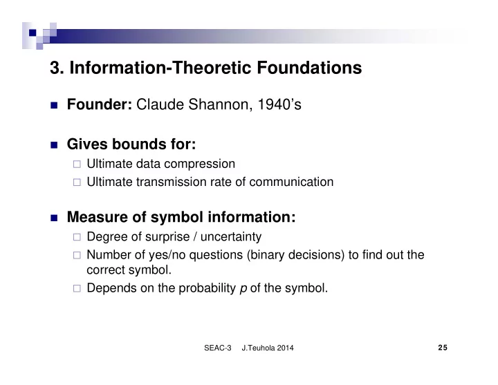
• 3. Information-Theoretic Foundations

Founder: Claude Shannon, 1940’s Gives bounds for:

Ultimate data compression Ultimate transmission rate of communication

Measure of symbol information:

Degree of surprise / uncertainty Number of yes/no questions (binary decisions) to find out the

correct symbol.

Depends on the probability p of the symbol.

SEAC-3 J.Teuhola 2014 26

Choosing the information measure

Requirements for information function I(p):

I(p) ≥ 0 I(p1p2) = I(p1) + I(p2) I(p) is continuous with p.

The solution is essentially unique:

I(p) = −log p = log (1/p).

Base of log = 2 ⇒ The unit of information is bit.

SEAC-3 J.Teuhola 2014 27

Examples

Tossing a fair coin: P(heads) = P(tails) = ½

Information measures for one toss:

Inf(heads) = Inf(tails) = -log20.5 bits = 1 bit

Information measure for a 3-sequence:

Inf(<heads, tails, heads>) = -log2(½⋅½⋅½) bits = 3 bits.

Optimal coding: heads 0, tails 1

An unfair coin: P(heads) = 1/8 and P(tails) = 7/8.

Inf(heads) = -log2(1/8) bits = 3 bits Inf(tails) = -log2(7/8) bits ≈ 0.193 bits Inf(<tails, tails, tails>) = -log2(7/8)3 bits ≈ 0.578 bits Improving the coding requires grouping of tosses into blocks.

SEAC-3 J.Teuhola 2014 28

Entropy

Measures the average information of a symbol from

alphabet S having probability distribution P:

Noiseless source encoding theorem (C. Shannon):

Entropy H(S) gives a lower bound on the average code length L for any instantaneously decodable system.

∑ ∑

= =

⎟ ⎟ ⎠ ⎞ ⎜ ⎜ ⎝ ⎛ = =

q i i i q i i i

p p p I p S H

1 2 1

1 log ) ( ) (

SEAC-3 J.Teuhola 2014 29

Example case: Binary source

Two symbols, e.g. S = {0, 1},

probabilities p0 and p1 = 1−p0.

Entropy = p0 = 0.5, p1 = 0.5 H(S) = 1 p0 = 0.1, p1 = 0.9 H(S) ≈ 0.469 p0 = 0.01, p1 = 0.99 H(S) ≈ 0.081 The skewer the distribution, the smaller the entropy. Uniform distribution results in maximum entropy

2 2

1 1 log ) 1 ( 1 log p p p p − − +

SEAC-3 J.Teuhola 2014 30

Example case: Predictive model

HELLO WOR ?

Already processed ‘context’

• log20.01

≈ 6.644 bits

• log20.04

≈ 4.644 bits

• log20.95

≈ 0.074 bits Inf (bits) 0.01 ⋅ 6.644 ≈ 0.066 bits 0.01 M 0.04 ⋅ 4.644 ≈ 0.186 bits 0.04 D 0.95 ⋅ 0.074 ≈ 0.070 bits 0.95 L Weighted information Prob Next char Weighted sum ≈ 0.322 bits

SEAC-3 J.Teuhola 2014 31

Code redundancy

Average redundancy of a code (per symbol):

L − H(S).

Redundancy can be made = 0, if symbol probabilities are

negative powers of 2. (Note that −log2(2−i) = i )

Generally possible: Universal code: L ≤ c1·H(S) + c2 Asymptotically optimal code: c1 = 1

log log

2 2

1 1 1 p l p

i i i

⎛ ⎝ ⎜ ⎞ ⎠ ⎟ ≤ < ⎛ ⎝ ⎜ ⎞ ⎠ ⎟ +

SEAC-3 J.Teuhola 2014 32

Generalization: m-memory source

Conditional information: Conditional entropy for a given context: Global entropy over all contexts:

log ( ( | , , ))

2 1

1

P s s s

i i im

• H S s

s P s s s P s s s

i i i i i S i i i

m m m

( | , , ) ( | , , )log ( | , , )

1 1 1

2

1

• =

⎛ ⎝ ⎜ ⎜ ⎞ ⎠ ⎟ ⎟

∑

H S P s s P s s s P s s s P s s s P s s s

i i S S i i i i i i i i i S i i i

m m m m m m m

( ) ( , , ) ( | , , )log ( | , , ) ( , , , )log ( | , , ) = ⎛ ⎝ ⎜ ⎜ ⎞ ⎠ ⎟ ⎟ = ⎛ ⎝ ⎜ ⎜ ⎞ ⎠ ⎟ ⎟

∑ ∑ ∑

+ 1 1 1 1 1 1

2 2

1 1

SEAC-3 J.Teuhola 2014 33

About conditional sources

Generalized Markov process:

Finite-state machine For an m-memory source there are qm states Transitions correspond to symbols that follow the m-block Transition probabilities are state-dependent

Ergodic source:

System settles down to

a limiting probability distribution.

Equilibrium state probabilities

can be inferred from transition probabilities. 1 0.2 0.5 0.5 0.8

SEAC-3 J.Teuhola 2014 34

Solving the example entropy

∑∑

= =

= =

1 1

) | Pr( 1 log ) | Pr( ) (

i j i

i j i j p S H

1 0.2 0.5 0.5 0.8

893 . ) 5 . 1 log 5 . 5 . 1 log 5 . ( ) 8 . 1 log 8 . 2 . 1 log 2 . (

1

≈ + + + p p

1 1 1

5 . 8 . 5 . 2 . p p p p p p + = + =

Solution: eigenvector p0 = 0.385, p1 = 0.615 Example application: compression of black-and – white images (black and white areas highly clustered)

SEAC-3 J.Teuhola 2014 35

Empirical observations

Shannon’s experimental value for the entropy of the

English language ≈ 1 bit per character

Current text compressor efficiencies:

gzip ≈ 2.5 – 3 bits per character bzip2 ≈ 2.5 bits per character The best predictive methods ≈ 2 bits per character

Improvements are still possible! However, digital images, audio and video are more

important data types from compression point of view.

SEAC-3 J.Teuhola 2014 36

Other extensions of entropy

Joint entropy, e.g. for two random variables X, Y: Relative entropy: difference of using qi instead of pi: Differential entropy for continuous probability distribution:

∑

− =

y x y x y x

p p Y X H

, , 2 , log

) , (

∑

=

i i i i KL

q p p Q P D

2

log ) || (

∫

− =

X

dx x f x f X h ) ( log ) ( ) (

SEAC-3 J.Teuhola 2014 37

Kolmogorov complexity

Measure of message information = Length of the

shortest binary program for generating the message.

This is close to entropy H(S) for a sequence of symbols

drawn at random from a distribution that S has.

Can be much smaller than entropy for artificially

generated data: pseudo random numbers, fractals, ...

Problem: Kolmogorov complexity is not computable!

(Cf. Gödel’s incompleteness theorem and Turing machine stopping problem).