3.1 Introduction to Determinants McDonald Fall 2018, MATH 2210Q, - PDF document
NOTE: These slides contain both Sections 3.1 and 3.2. 3.1 Introduction to Determinants McDonald Fall 2018, MATH 2210Q, 3.1&3.2 Slides 3.1 Homework : Read section and do the reading quiz. Start with practice problems. Hand in : 4, 8, 13,
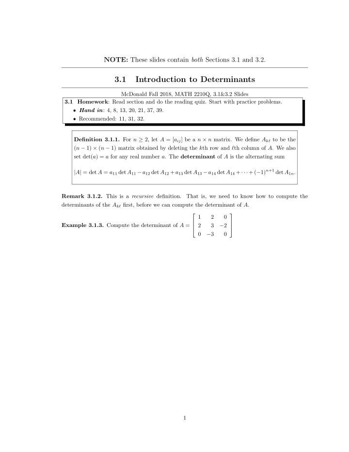
NOTE: These slides contain both Sections 3.1 and 3.2. 3.1 Introduction to Determinants McDonald Fall 2018, MATH 2210Q, 3.1&3.2 Slides 3.1 Homework : Read section and do the reading quiz. Start with practice problems. ❼ Hand in : 4, 8, 13, 20, 21, 37, 39. ❼ Recommended: 11, 31, 32. Definition 3.1.1. For n ≥ 2, let A = [ a ij ] be a n × n matrix. We define A kℓ to be the ( n − 1) × ( n − 1) matrix obtained by deleting the k th row and ℓ th column of A . We also set det( a ) = a for any real number a . The determinant of A is the alternating sum | A | = det A = a 11 det A 11 − a 12 det A 12 + a 13 det A 13 − a 14 det A 14 + · · · + ( − 1) n +1 det A 1 n . Remark 3.1.2. This is a recursive definition. That is, we need to know how to compute the determinants of the A kℓ first, before we can compute the determinant of A . 1 2 0 Example 3.1.3. Compute the determinant of A = 2 3 − 2 0 − 3 0 1
Definition 3.1.4. Given A = [ a ij ], the ( i, j ) -cofactor of A is the number C ij = ( − 1) i + j det A ij Theorem 3.1.5. The determinant of an n × n matrix A can be computed by a cofactor expansion across any row or down any column. The expansion of across the i th row is | A | = det A = a i 1 C i 1 + a i 2 C i 2 + · · · + a in C in . The cofactor expansion down the j th column is | A | = det A = a 1 j C 1 j + a 2 j C 2 j + · · · + a nj C nj . Example 3.1.6. Use a cofactor expansion across the third row to compute det A where 1 2 0 A = 2 3 − 2 0 − 3 0 2
3 1 − 2 6 1 0 2 5 − 2 3 Example 3.1.7. Compute the determinant of A = 0 0 1 2 0 0 0 2 3 − 2 0 0 0 − 3 0 Theorem 3.1.8. If A is an n × n triangular matrix, then det A = a 11 a 22 a 33 · · · a nn . Remark 3.1.9. This suggests a nice strategy. Turn A into a triangular matrix! We could try to reduce A to echelon form, U . How are determinants affected by row operations? 3
3.2 Properties of Determinants 3.2 Homework : Read section and do the reading quiz. Start with practice problems. ❼ Hand in : 8, 10, 16, 17, 20, 27, 34. ❼ Recommended: 2, 3, 26, 32, 40. Theorem 3.2.1 (Row Operations) . Let A be a square matrix. (a) If a multiple of one row of A is added to another to produce B , then det B = det A . (b) If two rows of A are interchanged to produce B , then det B = − det A . (c) If one row of A is multiplied by k to produce B , then det B = k det A . 1 − 4 2 Example 3.2.2. Compute det A where A = − 2 8 − 9 − 1 7 0 4
2 − 8 6 8 3 − 9 5 10 Example 3.2.3. Compute det A , where A = . − 3 0 1 − 2 1 − 4 0 6 Suppose an n × n matrix A can be reduced to echelon form U using only row replacements and row interchanges. Since U is in echelon form, it is triangular, so det U = u 11 u 22 u 33 · · · u nn . Proposition 3.2.4. If an n × n matrix A can be reduced to echelon form U using only row replacements and k row interchanges, then det A = ( − 1) k u 11 u 22 u 33 · · · u nn . 5
Theorem 3.2.5. A square matrix A is invertible if and only if det A � = 0 . 3 − 1 2 − 5 0 5 − 3 − 6 Example 3.2.6. Compute det A , where A = . − 6 7 − 7 4 − 5 − 8 0 9 0 1 2 − 1 2 5 − 7 3 Example 3.2.7. Compute det A , where A = . 0 3 6 2 − 2 − 5 4 − 2 6
Theorem 3.2.8. If A and B are n × n matrices, then det AB = (det A )(det B ) . � � � � 1 0 1 2 Example 3.2.9. Verify Theorem 3.2.8 for A = and B = . 2 5 3 4 Example 3.2.10. Let A and P be square matrices with P invertible, and show that det( PAP − 1 ) = det A . 7
Theorem 3.2.11. If A is an n × n matrix, then det A T = det A . Remark 3.2.12. This means we can perform operations on the columns of a matrix in the same way that we perform row operations, and expect the same effect on the determinant. − 5 2 2 2 3 0 3 5 Example 3.2.13. Compute det A , where A = . − 4 0 4 0 − 2 0 2 − 2 Theorem 3.2.14 (“Column” Operations) . Let A be a square matrix. (a) If a multiple of one column of A is added to another to produce B , then det B = det A . (b) If two columns of A are interchanged to produce B , then det B = − det A . (c) If one column of A is multiplied by k to produce B , then det B = k det A . 8
Recommend
More recommend
Explore More Topics
Stay informed with curated content and fresh updates.















![The Determinant of a Square Matrix [AR 2.12.3] The row vectors of an n n matrix a](https://c.sambuz.com/997829/the-determinant-of-a-square-matrix-ar-2-1-2-3-s.webp)