( ) 2017.04.27 CS686 Presentation #1 Bircher, Andreas, et al. - PowerPoint PPT Presentation
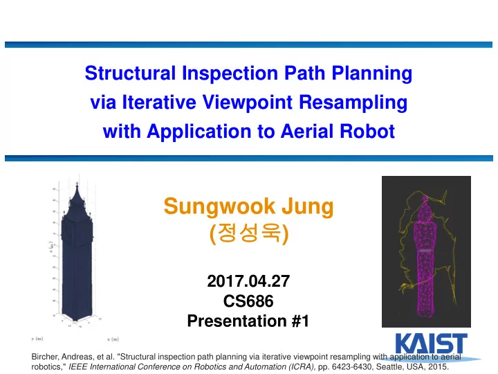
Structural Inspection Path Planning via Iterative Viewpoint Resampling with Application to Aerial Robot Sungwook Jung ( ) 2017.04.27 CS686 Presentation #1 Bircher, Andreas, et al. "Structural inspection path planning via
Structural Inspection Path Planning via Iterative Viewpoint Resampling with Application to Aerial Robot Sungwook Jung ( 정성욱 ) 2017.04.27 CS686 Presentation #1 Bircher, Andreas, et al. "Structural inspection path planning via iterative viewpoint resampling with application to aerial robotics," IEEE International Conference on Robotics and Automation (ICRA), pp. 6423-6430, Seattle, USA, 2015.
Introduction ● In the fields of inspection operations, ● autonomous complete coverage 3D structural path planning is required. ● A robot needs quick algorithms that result in full coverage of the structure while respecting any sensor limitations and motion constraints. ● A novel fast algorithm that provides efficient solutions to the problem of inspection path planning for complex 3D structures is proposed 2
Problem description ● Conventional 3D methods: ● Two-step optimization 1. Compute the minimal set of viewpoints that cover whole structure (solving Art Gallery Problem (AGP[1])). 2. Compute the shortest connecting tour over these viewpoints (Travelling Salesman Problem (TSP[2])). Large cost of computing efficiency ● They are prone to be suboptimal due to the two-step ● separation of the problem. In specific cases they can lead to unfeasible solutions/paths ● (e.g. in the case of non-holonomic vehicles) [1] J. O’rourke , Art gallery theorems and algorithms. Oxford University Press Oxford, 1987, vol. 57. [2] G. Dantzig , R. Fulkerson, and S. Johnson, “Solution of a large - scale traveling- salesman problem,” 3 Journal of the operations research society of America, vol. 2, no. 4, pp. 393 – 410, 1954.
Contributions ● Not minimizing the number of viewpoints, it samples them such that connecting path is short while ensuring full coverage ● A two step optimization paradigm to find good viewpoints that together provide full coverage and a connecting path that has low cost ● First: In every iteration, each viewpoints is chosen to reduce the cost-to-travel between itself and its neighbors ● Second: the optimally connecting tour is recomputed 4
Methodology: psedo-code Algorithm 1 Inspection path planner First solution 1. Load the mesh model 2. k = 0 3. Sample Initial Viewpoint Configurations (Viewpoint Sampler) 4. Find a Collision-free path for all possible viewpoint combinations (boundary value solver (BVS), RRT*) 5. Populate the Cost Matrix and Solve the Traveling Salesman Problem (Lin-Kernighan- Helsgaun Heuristic (LKH)) 6. while running Optimized solution 1. Re-sample Viewpoint Configurations (Viewpoint Sampler) 2. Re-compute the Collision-free paths (BVS, RRT*) 3. Re-populate the Cost Matrix and solve the new Traveling Salesman Problem to update the current best inspection tour (LKH) 4. k = k + 1 7. end while 8. Return BestTour, CostBestTour 5
ሶ path computation Methodology: and cost estimation ● To find the best tour among viewpoints, TSP solver requires a cost matrix of all pairs of viewpoints ● Path generation and cost estimation is done by either ● BVS - directly connect the two viewpoints ● BVS+RRT* - due to obstacles, connection is not feasible ● The cost of a path segment corresponds to the execution time 𝒖 𝒇𝒚 Τ Τ • 𝒖 𝒇𝒚 = 𝐧𝐛𝐲 𝒆 𝒘 𝒏𝒃𝒚 , 𝝎 𝟐 − 𝝎 𝟏 𝝎 𝒏𝒃𝒚 Where 𝒆 is the Euclidean distance, translation speed limit is 𝒘 𝒏𝒃𝒚 , rotational speed limit is ሶ 𝝎 𝒏𝒃𝒚 , and 𝝎 is yaw angle, respectively 6
Methodology: viewpoint sampling ● For every triangle in the mesh, one viewpoint has to be sampled, the position and heading is determined while retaining visibility of the corresponding triangle. ● First, the position is optimized for distance to the neighboring viewpoints using a convex problem formulation and then heading is optimized. ● To guarantee a good result, the position solution must be constrained such as to allow finding an orientation for which the triangle is visible. 7
Methodology: viewpoint sampling ● The constraints on the position 𝒉 = [𝒚, 𝒛, 𝒜] consist of the inspection sensor limitation of minimum incidence angle, minimum and maximum range (𝒆 𝒏𝒋𝒐 , 𝒆 𝒏𝒃𝒚 ) constraints. ● Where 𝒚 𝒋 are the corner of the mesh triangle, 𝒃 𝑶 is the normalized triangle ● normal and 𝒚 𝒋 are the normal of the separating hyperplanes for incidence angle constraints, respectively. Three main planar angle of incidence constraints on all three sides of the triangle. For a finite number of such constraints the incidence angle is only enforced approximately. The red line (and 𝒐 + ) demarks a sample orientation for a possible additional planar constraint at a corner. Minimum (green plane) and maximum (red plane) distance constraints are similar planar constraints on the sampling area. These constraints bound the sampling space, where g can be chosen, on all sides (gray area). b) Incidence angle constraints on a triangular facet 8
Methodology: viewpoint sampling ● To account for the limited FoV with fixed pitch angle of camera, it imposes a revoluted 2D-cone constraint which is nonconvex problem and then convexified by dividing the space into 𝑶 𝑫 equal convex pieces. ● The optimum is computed for every slice. where 𝒚 𝒎𝒑𝒙𝒇𝒔 𝒔𝒇𝒎 , 𝒚 𝒗𝒒𝒒𝒇𝒔 are the respective relevant corners of • 𝒔𝒇𝒎 𝒅𝒃𝒏 , the mesh triangle, m the middle of the triangle and 𝒐 𝒎𝒑𝒙𝒇𝒔 𝒅𝒃𝒏 , 𝒐 𝒔𝒋𝒉𝒊𝒖 and 𝒐 𝒎𝒇𝒈𝒖 denote the normal of the respective 𝒐 𝒗𝒒𝒒𝒇𝒔 separating hyperplanes. 9
Methodology: viewpoint sampling ● Optimization objective is to minimize the sum of squared distances to the preceding viewpoint 𝒉 𝒒 𝒍−𝟐 , the subsequent 𝒍−𝟐 and the current viewpoint in the old tour 𝒉 𝒍−𝟐 . viewpoint 𝒉 𝒕 ● The heading is determined according to 10
Computational Analysis ● To evaluate the capabilities, a simple scenario is used. Facets variable incidence 30° FoV [70,70] ° Mounting pitch 25° 200m 200m 𝒆 𝒏𝒋𝒐 𝒆 𝒏𝒃𝒚 5m/s 0.5rad/s 𝒘 𝒏𝒃𝒚 𝝎 𝒏𝒃𝒚 The time complexity: LKH: 𝑷(𝑶 𝟑.𝟑 ) VP Sampling: 𝑷(𝑶) Correlation of the number of viewpoints with Distance compute.: 𝑷(𝑶 𝟑 ) the computational time consumption. 11
Evaluation Test - Simulation ● 405m Tower Large scale structure to be inspected: The 405m high Central Radio & TV Tower in Beijing. The mesh used to compute the path contains 1701 triangular facets. After a computation time of 92s the cost for the inspection is 2997.44s The red point denotes, start – and end – point of the inspection. 12
Evaluation Test – VTOL UAV ● Online: image processing ● Offline: 3D reconstruction (Image->Pix4D) Path planner Visual-Inertial Sensor, ● Cost for the inspection: 151.44s ATOM CPU (Linux) 13
Self-test: solar plant 14
Self-test: Bigben 15
Summary & Conclusions ● A practically – oriented fast inspection path planning algorithm capable of computing efficient solutions for complex 3Dstructures represented by triangular meshes was presented. ● With the help of 3D reconstruction software, the recorded inspection data were post-processed to support the claim of finding full coverage paths and the point cloud datasets are released to enable evaluation of the inspection quality. ● https://github.com/ethz-asl/StructuralInspectionPlanner 16
● Thanks 17
Appendix.1 ● Art Gallery Problem (AGP) Suppose you have an art gallery containing priceless paintings and sculptures. You would like it to be supervised by security guards, and you want to employ enough of them so that at any one time the guards can between them oversee the whole gallery. How many guards will you need? ● Travelling Salesman Problem (TSP) Given a list of cities and the distances between each pair of cities, what is the shortest possible route that visits each city exactly once and returns to the origin city? 18
Appendix.2 ● Boundary Value Problem (or Solution) ● A boundary value problem has conditions specified at the extremes ("boundaries") of the independent variable in the equation ● whereas an initial value problem has all of the conditions specified at the same value of the independent variable (and that value is at the lower boundary of the domain, thus the term "initial" value). 19
Appendix.3 ● Lin-Kernighan-Helsgaun heuristic (LKH, K. Helsgaun, 1998) ● LKH is an effective implementation of the Lin- Kernighan heuristic for solving the traveling salesman problem. ● Even though the algorithm is approximate, optimal solutions are produced with an impressively high frequency. ● Employs the concept of k-opt moves Visualization of the k-moves process 20
Recommend
More recommend
Explore More Topics
Stay informed with curated content and fresh updates.
