2012 NCTS Workshop on Dynamical Systems National Center for - PowerPoint PPT Presentation
Deterministic SlowFast Systems Slowly driven systems Fully coupled systems Deterministic averaging Random fast motion 2012 NCTS Workshop on Dynamical Systems National Center for Theoretical Sciences, National Tsing-Hua University Hsinchu,
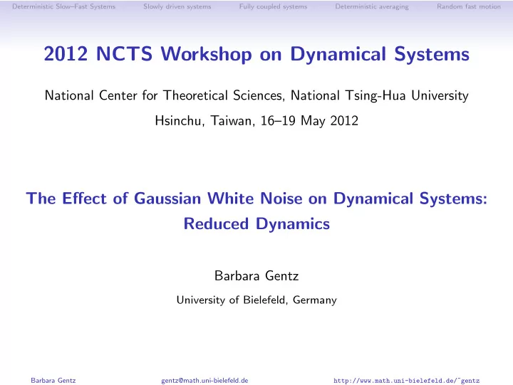
Deterministic Slow–Fast Systems Slowly driven systems Fully coupled systems Deterministic averaging Random fast motion 2012 NCTS Workshop on Dynamical Systems National Center for Theoretical Sciences, National Tsing-Hua University Hsinchu, Taiwan, 16–19 May 2012 The Effect of Gaussian White Noise on Dynamical Systems: Reduced Dynamics Barbara Gentz University of Bielefeld, Germany Barbara Gentz gentz@math.uni-bielefeld.de http://www.math.uni-bielefeld.de/ ˜ gentz
Deterministic Slow–Fast Systems Slowly driven systems Fully coupled systems Deterministic averaging Random fast motion General slow–fast systems Reduced Dynamics Barbara Gentz NCTS, 17 May 2012 1 / 29
Deterministic Slow–Fast Systems Slowly driven systems Fully coupled systems Deterministic averaging Random fast motion General slow–fast systems Fully coupled SDEs on well-separated time scales d x t = 1 ε f ( x t , y t ) d t + σ √ ε F ( x t , y t ) d W t (fast variables ∈ R n ) g ( x t , y t ) d t + σ ′ G ( x t , y t ) d W t d y t = (slow variables ∈ R m ) ⊲ { W t } t ≥ 0 k -dimensional (standard) Brownian motion ⊲ D ⊂ R n × R m ⊲ f : D → R n , g : D → R m drift coefficients, ∈ C 2 ⊲ F : D → R n × k , G : D → R m × k diffusion coefficients, ∈ C 1 Small parameters ⊲ ε > 0 adiabatic parameter ( no quasistatic approach) ⊲ σ, σ ′ ≥ 0 noise intensities; may depend on ε : σ = σ ( ε ), σ ′ = σ ′ ( ε ) and σ ′ ( ε ) /σ ( ε ) = ̺ ( ε ) ≤ 1 Reduced Dynamics Barbara Gentz NCTS, 17 May 2012 2 / 29
Deterministic Slow–Fast Systems Slowly driven systems Fully coupled systems Deterministic averaging Random fast motion Singular limits for deterministic slow–fast systems In slow time t In fast time s = t /ε t �→ s x ′ = f ( x , y ) ⇐ ⇒ ε ˙ x = f ( x , y ) y ′ = ε g ( x , y ) y = g ( x , y ) ˙ � ε → 0 � ε → 0 Slow subsystem Fast subsystem x ′ = f ( x , y ) 0 = f ( x , y ) ⇐ / ⇒ y ′ = 0 y = g ( x , y ) ˙ Study slow variable y on slow Study fast variable x for frozen manifold f ( x , y ) = 0 slow variable y Reduced Dynamics Barbara Gentz NCTS, 17 May 2012 3 / 29
Deterministic Slow–Fast Systems Slowly driven systems Fully coupled systems Deterministic averaging Random fast motion Near slow manifolds: Assumptions on the fast variables ⊲ Existence of a slow manifold ∃ x ⋆ : D 0 → R n ∃ D 0 ⊂ R m s.t. ( x ⋆ ( y ) , y ) ∈ D and f ( x ⋆ ( y ) , y ) = 0 for y ∈ D 0 ⊲ Slow manifold is attracting Eigenvalues of A ⋆ ( y ) := ∂ x f ( x ⋆ ( y ) , y ) satisfy Re λ i ( y ) ≤ − a 0 < 0 (uniformly in D 0 ) Reduced Dynamics Barbara Gentz NCTS, 17 May 2012 4 / 29
Deterministic Slow–Fast Systems Slowly driven systems Fully coupled systems Deterministic averaging Random fast motion Fenichel’s theorem Theorem ([Tihonov ’52, Fenichel ’79]) There exists an adiabatic manifold : ∃ ¯ x ( y , ε ) s.t. ⊲ ¯ x ( y , ε ) is invariant manifold for deterministic dynamics ⊲ ¯ x ( y , ε ) attracts nearby solutions ⊲ ¯ x ( y , 0) = x ⋆ ( y ) ⊲ ¯ x ( y , ε ) = x ⋆ ( y ) + O ( ε ) ¯ x ( y , ε ) x ⋆ ( y ) x y 2 y 1 Consider now stochastic system under these assumptions Reduced Dynamics Barbara Gentz NCTS, 17 May 2012 5 / 29
Deterministic Slow–Fast Systems Slowly driven systems Fully coupled systems Deterministic averaging Random fast motion Random slow–fast systems: Slowly driven systems Reduced Dynamics Barbara Gentz NCTS, 17 May 2012 6 / 29
Deterministic Slow–Fast Systems Slowly driven systems Fully coupled systems Deterministic averaging Random fast motion Typical neighbourhoods for the stochastic fast variable Special case: One-dim. slowly driven systems d x t = 1 ε f ( x t , t ) d t + σ √ ε d W t Stable slow manifold / stable equilibrium branch x ⋆ ( t ): f ( x ⋆ ( t ) , t ) = 0 , a ⋆ ( t ) = ∂ x f ( x ⋆ ( t ) , t ) � − a 0 < 0 x ( t , ε ) ≈ x ⋆ ( t ) Linearize SDE for deviation x t − ¯ x ( t , ε ) from adiabatic solution ¯ d z t = 1 ε a ( t ) z t d t + σ √ ε d W t We can solve the non-autonomous SDE for z t � t z t = z 0 e α ( t ) /ε + σ e α ( t , s ) /ε d W s √ ε 0 � t where α ( t ) = a ( s ) d s , α ( t , s ) = α ( t ) − α ( s ) and a ( t ) = ∂ x f (¯ x ( t , ε ) , t ) 0 Reduced Dynamics Barbara Gentz NCTS, 17 May 2012 7 / 29
Deterministic Slow–Fast Systems Slowly driven systems Fully coupled systems Deterministic averaging Random fast motion Typical spreading � t z t = z 0 e α ( t ) /ε + σ e α ( t , s ) /ε d W s √ ε 0 z t is a Gaussian r.v. with variance � t v ( t ) = Var( z t ) = σ 2 σ 2 e 2 α ( t , s ) /ε d s ≈ ε | a ( t ) | 0 � For any fixed time t , z t has a typical spreading of v ( t ), and a standard estimate shows P {| z t | ≥ h } ≤ e − h 2 / 2 v ( t ) Goal: Similar concentration result for the whole sample path � Define a strip B ( h ) around ¯ x ( t , ε ) of width ≃ h / | a ( t ) | � B ( h ) = { ( x , t ): | x − ¯ x ( t , ε ) | < h / | a ( t ) |} Reduced Dynamics Barbara Gentz NCTS, 17 May 2012 8 / 29
Deterministic Slow–Fast Systems Slowly driven systems Fully coupled systems Deterministic averaging Random fast motion Concentration of sample paths x ⋆ ( t ) x t ¯ x ( t , ε ) B ( h ) Theorem [Berglund & G ’02, ’06] � t � 2 1 � h � � σ e − h 2 [1 −O ( ε ) −O ( h )] / 2 σ 2 � � x t leaves B ( h ) before time t ≃ a ( s ) d s P � � π ε � 0 Reduced Dynamics Barbara Gentz NCTS, 17 May 2012 9 / 29
Deterministic Slow–Fast Systems Slowly driven systems Fully coupled systems Deterministic averaging Random fast motion Fully coupled random slow–fast systems Reduced Dynamics Barbara Gentz NCTS, 17 May 2012 10 / 29
Deterministic Slow–Fast Systems Slowly driven systems Fully coupled systems Deterministic averaging Random fast motion Typical spreading in the general case d x t = 1 ε f ( x t , y t ) d t + σ (fast variables ∈ R n ) √ ε F ( x t , y t ) d W t g ( x t , y t ) d t + σ ′ G ( x t , y t ) d W t d y t = (slow variables ∈ R m ) ⊲ Consider det. process ( x det x ( y det , ε ) , y det = ¯ ) on adiabatic manifold t t t ⊲ Deviation ξ t := x t − x det of fast variables from adiabatic manifold t ⊲ Linearize SDE for ξ t ; resulting process ξ 0 t is Gaussian Key observation 1 σ 2 Cov ξ 0 t is a particular solution of the deterministic slow–fast system ) X ( t ) + X ( t ) A ( y det ) T + F 0 ( y det ) F 0 ( y det ) T ε ˙ X ( t ) = A ( y det � t ( ∗ ) y det x ( y det , ε ) , y det ˙ = g (¯ ) t t t with A ( y ) = ∂ x f (¯ x ( y , ε ) , y ) and F 0 0 th -order approximation to F Reduced Dynamics Barbara Gentz NCTS, 17 May 2012 11 / 29
Deterministic Slow–Fast Systems Slowly driven systems Fully coupled systems Deterministic averaging Random fast motion Typical neighbourhoods in the general case Typical neighbourhoods , X ( y , ε ) − 1 � < h 2 � � �� � �� B ( h ) := ( x , y ): x − ¯ x ( y , ε ) x − ¯ x ( y , ε ) where X ( y , ε ) denotes the adiabatic manifold for the system ( ∗ ) B ( h ) Reduced Dynamics Barbara Gentz NCTS, 17 May 2012 12 / 29
Deterministic Slow–Fast Systems Slowly driven systems Fully coupled systems Deterministic averaging Random fast motion Concentration of sample paths Define (random) first-exit times τ D 0 := inf { s > 0: y s / ∈ D 0 } τ B ( h ) := inf { s > 0: ( x s , y s ) / ∈ B ( h ) } Theorem [Berglund & G, JDE 2003] Assume � X ( y , ε ) � , � X ( y , ε ) − 1 � uniformly bounded in D 0 Then ∃ ε 0 > 0 ∃ h 0 > 0 ∀ ε � ε 0 ∀ h � h 0 − h 2 � �� � � � P τ B ( h ) < min( t , τ D 0 ) � C n , m ( t ) exp 1 − O ( h ) − O ( ε ) 2 σ 2 C m + h − n �� 1 + t � � where C n , m ( t ) = ε 2 Reduced Dynamics Barbara Gentz NCTS, 17 May 2012 13 / 29
Deterministic Slow–Fast Systems Slowly driven systems Fully coupled systems Deterministic averaging Random fast motion Reduced dynamics Reduction to adiabatic manifold ¯ x ( y , ε ): d y 0 x ( y 0 t , ε ) , y 0 x ( y 0 t , ε ) , y 0 t ) d t + σ ′ G (¯ t = g (¯ t ) d W t Theorem – informal version [Berglund & G ’06] t approximates y t to order σ √ ε up to Lyapunov time of ˙ y det = g (¯ y 0 x ( y det , ε ) y det ) Remark For σ ′ σ < √ ε , the deterministic reduced dynamics provides a better approximation Reduced Dynamics Barbara Gentz NCTS, 17 May 2012 14 / 29
Deterministic Slow–Fast Systems Slowly driven systems Fully coupled systems Deterministic averaging Random fast motion Longer time scales Behaviour of g or behaviour of y t and y det becomes important t Example: y det following a stable periodic orbit t const ⊲ y t ∼ y det for t � σ ∨ ̺ 2 ∨ ε t linear coupling → ε nonlinear coupling → σ noise acting on slow variable → ̺ ⊲ On longer time scales: Markov property allows for restarting y t stays exponentially long in a neighbourhood of the periodic orbit (with probability close to 1) Reduced Dynamics Barbara Gentz NCTS, 17 May 2012 15 / 29
Deterministic Slow–Fast Systems Slowly driven systems Fully coupled systems Deterministic averaging Random fast motion The main idea of deterministic averaging Reduced Dynamics Barbara Gentz NCTS, 17 May 2012 16 / 29
Recommend
More recommend
Explore More Topics
Stay informed with curated content and fresh updates.
