2.5 Association Rule Mining based on: Chlo e-Agathe Azencott and - PowerPoint PPT Presentation

2.5 Association Rule Mining based on: Chlo´ e-Agathe Azencott and Karsten Borgwardt. Course ’Data Mining in Bioinformatics’. Chapter Graph Mining. 2012 Department Biosysteme Karsten Borgwardt Data Mining 2 Course, Basel Spring Semester 2016 179 / 230

Keyword co-occurrence Goals To understand the link between keyword co-occurrence, and association rule mining and frequent itemset mining To understand how the computation of frequent itemsets can be sped up Department Biosysteme Karsten Borgwardt Data Mining 2 Course, Basel Spring Semester 2016 180 / 230

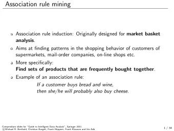
Keyword co-occurrence Problem Find sets of keyword that often co-occur Common problem in biomedical literature: find associations between genes, proteins or other entities using co-occurrence search Keyword co-occurrence search is an instance of a more general problem in data mining, called association rule mining. Department Biosysteme Karsten Borgwardt Data Mining 2 Course, Basel Spring Semester 2016 181 / 230

Association Rules Definitions Let I = { I 1 , I 2 , . . . , I m } be a set of items (keywords) Let D be the database of transactions T (collection of documents) A transaction T ∈ D is a set of items: T ⊆ I (a document is a set of keywords) Let A be a set of items: A ⊆ T . An association rule is an implication of the form A ⊆ T ⇒ B ⊆ T , (1) where A , B ⊆ I and A ∩ B = ∅ Department Biosysteme Karsten Borgwardt Data Mining 2 Course, Basel Spring Semester 2016 182 / 230

Association Rules Support and Confidence The rule A ⇒ B holds in the transaction set D with support s , where s is the percentage of transactions in D that contain A ∪ B : support( A ⇒ B ) = |{ T ∈ D | A ⊆ T ∧ B ⊆ T }| (2) |{ T ∈ D }| The rule A ⇒ B has confidence c in the transaction set D , where c is the percentage of transactions in D containing A that also contain B : confidence( A ⇒ B ) = |{ T ∈ D | A ⊆ T ∧ B ⊆ T }| (3) |{ T ∈ D | A ⊆ T }| Department Biosysteme Karsten Borgwardt Data Mining 2 Course, Basel Spring Semester 2016 183 / 230

Association Rules Strong rules Rules that satisfy both a minimum support threshold (minsup) and a minimum confidence threshold (minconf) are called strong association rules — and these are the ones we are after! Finding strong rules 1. Search for all frequent itemsets (set of items that occur in at least minsup % of all transactions) 2. Generate strong association rules from the frequent itemsets Department Biosysteme Karsten Borgwardt Data Mining 2 Course, Basel Spring Semester 2016 184 / 230

Association Rules: Frequent pattern mining Frequent item set mining Market basket analysis Find items that are frequently purchased together Given a set B = { i 1 , i 2 , . . . , i n } of items a list T = { t 1 , t 2 , . . . , t m } of transactions t j ⊆ B a minimum number of occurences s min ∈ N Find the set of frequent item sets , i.e. F ( s min ) = { I ⊆ B : |{ k : I ⊆ t k } ≥ s min } Department Biosysteme Karsten Borgwardt Data Mining 2 Course, Basel Spring Semester 2016 185 / 230

Association Rules: Apriori [Agrawal et al. , 1994] Brute force approach Enumerate all 2 n subsets of B Count how often each of them is included in each of t 1 , . . . , t m Generally infeasible The Apriori property If an itemset A is frequent, then any subset B of A ( B ⊆ A ) is frequent as well. If B is infrequent, then any superset A of B ( A ⊇ B ) is infrequent as well. Department Biosysteme Karsten Borgwardt Data Mining 2 Course, Basel Spring Semester 2016 186 / 230

Association Rules Apriori Pseudocode 1 Determine frequent items = k -itemsets with k = 1 2 Join all pairs of frequent k -itemsets that differ in at most 1 item = candidates C k +1 for being frequent k + 1 itemsets 3 Check the frequency of these candidates C k +1 : the frequent ones form the frequent k + 1-itemsets (trick: discard any candidate immediately that contains an infrequent k -itemset) 4 Repeat from Step 2 until no more candidate is frequent. Department Biosysteme Karsten Borgwardt Data Mining 2 Course, Basel Spring Semester 2016 187 / 230

Association Rules: A Priori Generating unique candidates There are k ! ways of generating a single set of k items Ensure we do it only once ⇒ Idea: assign a unique parent set to each set Canonical form The set of possible parents of an item set I is the set of its maximal proper subsets : { J ⊂ I | ∄ K : J ⊂ K ⊂ I } Put an ordering on B : i 1 < i 2 < · · · < i n Define the canonical parent of I as p c ( I ) = I \ { max a ∈ I a } Department Biosysteme Karsten Borgwardt Data Mining 2 Course, Basel Spring Semester 2016 188 / 230

Association Rules: A Priori Canonical code words code word for I ⊆ B : any word w on the alphabet B canonical code word of I w c ( I ): smallest of these words, in lexicographic order E.g. { a , c , b , e } → abce The canonical parent of I p c ( I ) is described by the longest proper prefix of w c ( I ). Prefix property : The longest proper prefix of a canonical code word is a canonical code word itself. Equivalently, any prefix of a canonical code word is a canonical code word itself. Department Biosysteme Karsten Borgwardt Data Mining 2 Course, Basel Spring Semester 2016 189 / 230

Association Rules: A Priori Candidate set generation From frequent item sets of size k − 1, construct item sets of size k by appending (frequent) items to their canonical code words Only do so for items greater than the last letter of the canonical code word abe → abef , abeg , ✘✘ abec ✘ Department Biosysteme Karsten Borgwardt Data Mining 2 Course, Basel Spring Semester 2016 190 / 230

Association Rules: A Priori Prefix tree a b c d ab ac ad bc bd cd abc abd acd bcd abcd Full prefix tree for B = { a , b , c , d } Department Biosysteme Karsten Borgwardt Data Mining 2 Course, Basel Spring Semester 2016 191 / 230

Association Rules: A Priori Pruning the prefix tree Only generate unique item sets A-priori property ⇒ Prune branches at infrequent items Size-based pruning T = {{ a , b } , { a , b , c } , { b , c } , a b c d 4 11 9 7 { b } , { b , d } , { d } , { a , c } , { b , c } , { d } , { a , c } , { b , c } , { b , c , d } , ab ac ad bc bd cd { d } , { b } , { b , c , d } , { b , c , d }} 2 2 0 7 4 3 abc abd acd bcd 3 1 0 0 abcd 0 Department Biosysteme Karsten Borgwardt Data Mining 2 Course, Basel Spring Semester 2016 192 / 230

Association Rules: Frequent Pattern Mining Exploring the search tree Breadth-First Search : find all frequent sets of size k before moving on to size k + 1 → A-priori Depth-First Search : find all frequent sets containing element a before moving on to those that contain b but do not contain a Advantage : divide-and-conquer strategy, requires less memory → Eclat, FP-growth ... Department Biosysteme Karsten Borgwardt Data Mining 2 Course, Basel Spring Semester 2016 193 / 230

Association Rules Summary Keyword co-occurrence is a way to mine relationships between concepts from text databases. It is an instance of association rule mining, which tries to find associations between the occurrences of sets of words. The classic algorithm for finding association rules is the Apriori algorithm, which enumerates all frequent itemsets in a branch-and-bound fashion. Department Biosysteme Karsten Borgwardt Data Mining 2 Course, Basel Spring Semester 2016 194 / 230

3. Graph Mining based on: Chlo´ e-Agathe Azencott and Karsten Borgwardt. Course ’Data Mining in Bioinformatics’. Chapter Graph Mining. 2012 Department Biosysteme Karsten Borgwardt Data Mining 2 Course, Basel Spring Semester 2016 195 / 230

Graphs are everywhere Coexpression network Social network Program flow Protein structure Chemical compound Department Biosysteme Karsten Borgwardt Data Mining 2 Course, Basel Spring Semester 2016 196 / 230

Mining graph data Graph comparison Example: Compare PPIN between species Graph classification / regression Predict properties of objects represented as graphs Example: Predict toxicity of molecular compound, functionality of protein Graph nodes classification / regression Predict properties of objects connected on a graph Example: Predict functionality of protein, classify pixels in remote sensing images Department Biosysteme Karsten Borgwardt Data Mining 2 Course, Basel Spring Semester 2016 197 / 230

Mining graph data Graph compression Representing graphs compactly Example: Store and mine web data Graph clustering Finding dense subnetworks of graphs Example: Find groups in social networks Link prediction Predicting relationships between nodes of the graph Example: Predict who should be added to your social network, predict interactions Department Biosysteme Karsten Borgwardt Data Mining 2 Course, Basel Spring Semester 2016 198 / 230

Graph pattern mining Graph pattern mining Find frequent / informative graph patterns Summarize patterns Approximate patterns Applications Finding biological conserved subnetworks Finding functional modules Program control flow analysis Intrusion detection Building blocks for graph classification, clustering, compression, comparison Department Biosysteme Karsten Borgwardt Data Mining 2 Course, Basel Spring Semester 2016 199 / 230

3.1 Frequent Subgraph Mining Department Biosysteme Karsten Borgwardt Data Mining 2 Course, Basel Spring Semester 2016 200 / 230