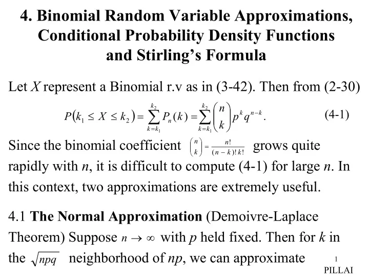

4. Binomial Random Variable Approximations, Conditional Probability Density Functions and Stirling’s Formula Let X represent a Binomial r.v as in (3-42). Then from (2-30) k k n ( ) ∑ 2 ∑ 2 (4-1) ≤ ≤ = = − k n k P k X k P ( k ) p q . 1 2 n k = = k k k k 1 1 Since the binomial coefficient grows quite n n ! = − k ( n k )! k ! rapidly with n , it is difficult to compute (4-1) for large n . In this context, two approximations are extremely useful. 4.1 The Normal Approximation (Demoivre-Laplace Theorem) Suppose with p held fixed. Then for k in → ∞ n the neighborhood of np , we can approximate npq 1 PILLAI
n 1 2 − − − ≈ k n k ( k np ) / 2 npq p q e . (4-2) π k 2 npq Thus if and in (4-1) are within or around the k k 2 1 ( ) , neighborhood of the interval we can − + np npq , np npq approximate the summation in (4-1) by an integration. In that case (4-1) reduces to 1 1 ( ) k x ∫ ∫ 2 2 (4-3) ≤ ≤ = − − = − 2 ( x np ) / 2 npq 2 y / 2 P k X k e dx e dy , 1 2 π π 2 npq 2 k x 1 1 where − − k np k np = = x 1 , x 2 . 1 2 npq npq We can express (4-3) in terms of the normalized integral 1 x (4-4) ∫ 2 = − = − y / 2 erf ( x ) e dy erf ( x ) π 2 0 that has been tabulated extensively (See Table 4.1). 2 PILLAI
For example, if and are both positive ,we obtain x x 2 1 ( ) (4-5) ≤ ≤ = − P k X k erf ( x ) erf ( x ). 1 2 2 1 Example 4.1: A fair coin is tossed 5,000 times. Find the probability that the number of heads is between 2,475 to 2,525. Solution: We need Here n is large so ≤ X ≤ P ( 2 , 475 2 , 525 ). 1 that we can use the normal approximation. In this case = p , 2 so that and Since − = = ≈ np 2 , 500 np npq 2 , 465 , npq 35 . and the approximation is valid for + = 1 = np npq 2 , 535 , k 2 , 475 and Thus 2 = k 2 , 525 . ) ∫ 1 ( x 2 − ≤ ≤ = 2 y / 2 P k X k e dy . 1 2 π 2 x 1 − − k np 5 k np 5 Here = = − = = x 1 , x 2 . 1 2 7 7 npq npq 3 PILLAI
1 1 x ∫ 2 = − = − y / 2 erf ( x ) e dy G ( x ) π 2 2 0 x erf( x ) x erf( x ) x erf( x ) x erf( x ) 0.05 0.01994 0.80 0.28814 1.55 0.43943 2.30 0.48928 0.10 0.03983 0.85 0.30234 1.60 0.44520 2.35 0.49061 0.15 0.05962 0.90 0.31594 1.65 0.45053 2.40 0.49180 0.20 0.07926 0.95 0.32894 1.70 0.45543 2.45 0.49286 0.25 0.09871 1.00 0.34134 1.75 0.45994 2.50 0.49379 0.30 0.11791 1.05 0.35314 1.80 0.46407 2.55 0.49461 0.35 0.13683 1.10 0.36433 1.85 0.46784 2.60 0.49534 0.40 0.15542 1.15 0.37493 1.90 0.47128 2.65 0.49597 0.45 0.17364 1.20 0.38493 1.95 0.47441 2.70 0.49653 0.50 0.19146 1.25 0.39435 2.00 0.47726 2.75 0.49702 0.55 0.20884 1.30 0.40320 2.05 0.47982 2.80 0.49744 0.60 0.22575 1.35 0.41149 2.10 0.48214 2.85 0.49781 0.65 0.24215 1.40 0.41924 2.15 0.48422 2.90 0.49813 0.70 0.25804 1.45 0.42647 2.20 0.48610 2.95 0.49841 0.75 0.27337 1.50 0.43319 2.25 0.48778 3.00 0.49865 Table 4.1 4 PILLAI
Since from Fig. 4.1(b), the above probability is given 1 < x 0 , ( ) by ≤ ≤ = − = + P 2 , 475 X 2 , 525 erf ( x ) erf ( x ) erf ( x ) erf (| x |) 2 1 2 1 5 = = 2 erf 0 . 516 , 7 ( ) . where we have used Table 4.1 = erf ( 0 . 7 ) 0 . 258 1 1 2 2 e − e − x / 2 x / 2 π π 2 2 x x x x x x 1 1 2 2 < > > > (b) x 0 , x 0 (a) x 0 , x 0 1 2 1 2 Fig. 4.1 4.2. The Poisson Approximation As we have mentioned earlier, for large n , the Gaussian approximation of a binomial r.v is valid only if p is fixed, i.e., only if and what if np is small, or if it >> >> np 1 npq 1 . does not increase with n ? 5 PILLAI
→ Obviously that is the case if, for example, as p 0 → ∞ n , = λ such that is a fixed number. np Many random phenomena in nature in fact follow this pattern. Total number of calls on a telephone line, claims in an insurance company etc. tend to follow this type of behavior. Consider random arrivals such as telephone calls over a line. Let n represent the total number of calls in the → ∞ interval From our experience, as we have → ∞ n ( 0 , T ). T = µ so that we may assume Consider a small interval of n T . duration ∆ as in Fig. 4.2. If there is only a single call coming in, the probability p of that single call occurring in that interval must depend on its relative size with respect to T . n 2 1 � ∆ 0 T 6 Fig. 4.2 PILLAI
∆ Hence we may assume Note that as → ∞ → = T . p . p 0 T ∆ However in this case is a constant, = µ ⋅ = µ ∆ = λ np T T and the normal approximation is invalid here. Suppose the interval ∆ in Fig. 4.2 is of interest to us. A call inside that interval is a “success” ( H ), whereas one outside is a “failure” ( T ). This is equivalent to the coin tossing situation, and hence the probability of obtaining k P n ( k ) calls (in any order) in an interval of duration ∆ is given by the binomial p.m.f. Thus n ! − = − (4-6) k n k P ( k ) p ( 1 p ) , n − ( n k )! k ! and here as such that It is easy to = λ → ∞ → np . n , p 0 obtain an excellent approximation to (4-6) in that situation. To see this, rewrite (4-6) as 7 PILLAI
− − + k n ( n 1 ) � ( n k 1 ) ( np ) − = − n k P ( k ) ( 1 np / n ) n k n k ! (4-7) − λ − λ k n − − 1 2 k 1 ( 1 / n ) = − 1 1 � 1 . − λ k n n n k ! ( 1 / n ) Thus λ k − λ = (4-8) lim P ( k ) e , n k ! → ∞ → = λ n , p 0 , np − 1 2 k 1 since the finite products as well − − − 1 1 � 1 n n n k − λ → ∞ as tend to unity as and n , 1 n n λ − λ − = lim 1 e . n → ∞ n The right side of (4-8) represents the Poisson p.m.f and the Poisson approximation to the binomial r.v is valid in situations where the binomial r.v parameters n and p → ∞ → diverge to two extremes such that their ( n , p 0 ) product np is a constant. 8 PILLAI
Example 4.2: Winning a Lottery: Suppose two million lottery tickets are issued with 100 winning tickets among them. (a) If a person purchases 100 tickets, what is the probability of winning? (b) How many tickets should one buy to be 95% confident of having a winning ticket? Solution: The probability of buying a winning ticket No. of winning tickets 100 − = = = × 5 p 5 10 . × 6 Total no. of tickets 2 10 Here and the number of winning tickets X in the n = n 100 , purchased tickets has an approximate Poisson distribution 5 = with parameter Thus − λ = = × × np 100 5 10 0 . 005 . λ k = = − λ P ( X k ) e , k ! and (a) Probability of winning = ≥ = − = = − −λ ≈ P ( X 1 ) 1 P ( X 0 ) 1 e 0 . 005 . 9 PILLAI
(b) In this case we need ≥ ≥ P ( X 1 ) 0 . 95 . ≥ = − − λ ≥ λ ≥ = P ( X 1 ) 1 e 0 . 95 implies ln 20 3 . 5 ≥ But or Thus one needs to λ = = × × − ≥ n 60 , 000 . np n 5 10 3 buy about 60,000 tickets to be 95% confident of having a winning ticket! ( ) → ∞ Example 4.3: A space craft has 100,000 components n The probability of any one component being defective is The mission will be in danger if five or × − → 5 2 10 ( p 0 ). more components become defective. Find the probability of such an event. Solution: Here n is large and p is small, and hence Poisson 5 = approximation is valid. Thus − = λ = × × np 100 , 000 2 10 2 , and the desired probability is given by 10 PILLAI
Recommend
More recommend