10c Machine Learning: Symbol-based 10.0 Introduction 10.5 - PowerPoint PPT Presentation
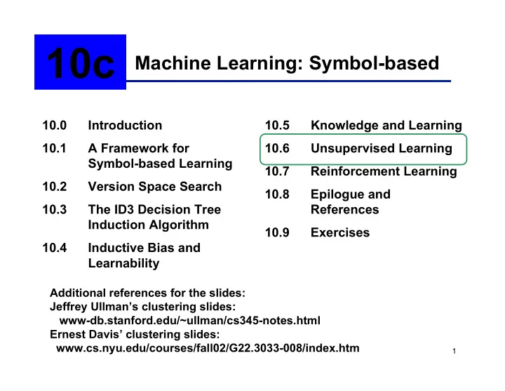
10c Machine Learning: Symbol-based 10.0 Introduction 10.5 Knowledge and Learning 10.1 A Framework for 10.6 Unsupervised Learning Symbol-based Learning 10.7 Reinforcement Learning 10.2 Version Space Search 10.8 Epilogue and 10.3 The
10c Machine Learning: Symbol-based 10.0 Introduction 10.5 Knowledge and Learning 10.1 A Framework for 10.6 Unsupervised Learning Symbol-based Learning 10.7 Reinforcement Learning 10.2 Version Space Search 10.8 Epilogue and 10.3 The ID3 Decision Tree References Induction Algorithm 10.9 Exercises 10.4 Inductive Bias and Learnability Additional references for the slides: Jeffrey Ullman’s clustering slides: www-db.stanford.edu/~ullman/cs345-notes.html Ernest Davis’ clustering slides: www.cs.nyu.edu/courses/fall02/G22.3033-008/index.htm 1
Unsupervised learning 2
Example: a cholera outbreak in London Many years ago, during a cholera outbreak in London, a physician plotted the location of cases on a map. Properly visualized, the data indicated that cases clustered around certain intersections, where there were polluted wells, not only exposing the cause of cholera, but indicating what to do about the problem. X X X X X X X X X X X X X X X X X X X X X 3
Conceptual Clustering The clustering problem Given • a collection of unclassified objects, and • a means for measuring the similarity of objects ( distance metric ), find • classes (clusters) of objects such that some standard of quality is met (e.g., maximize the similarity of objects in the same class.) Essentially, it is an approach to discover a useful summary of the data. 4
Conceptual Clustering (cont’d) Ideally, we would like to represent clusters and their semantic explanations. In other words, we would like to define clusters extensionally (i.e., by general rules) rather than intensionally (i.e., by enumeration). For instance, compare { X | X teaches AI at MTU CS}, and { John Lowther, Nilufer Onder} 5
Curse of dimensionality • While clustering looks intuitive in 2 dimensions, many applications involve 10 or 10,000 dimensions • High-dimensional spaces look different: the probability of random points being close drops quickly as the dimensionality grows 6
Higher dimensional examples • Observation that customers who buy diapers are more likely to buy beer than average allowed supermarkets to place beer and diapers nearby, knowing many customers would walk between them. Placing potato chips between increased the sales of all three items. 7
Skycat software 8
Skycat software (cont’d) • Skycat is a catalog of sky objects • Objects are represented by their radiation in 9 dimensions (each dimension represents radiation in one band of the spectrum • Skycat clustered 2 x 10 9 sky objects into similar objects e.g., stars, galaxies, quasars, etc. • The Sloan Sky Survey is a newer, better version to catalog and cluster the entire visible universe. Clustering sky objects by their radiation levels in different bands allowed astronomers to distinguish between galaxies, nearby stars, and many other kinds of celestial objects. 9
Clustering CDs • Intuition: music divides into categories and customers prefer a few categories • But what are categories really? • Represent a CD by the customers who bought it • Similar CDs have similar sets of customers and vice versa 10
The space of CDs • Think of a space with one dimension for each customer • Values in a dimension may be 0 or 1 only • A CD’s point in this space is (x 1 , x 2 , …, x n ) , where x i = 1 iff the i th customer bought the CD • Compare this with the correlated items matrix: rows = customers columns = CDs 11
Clustering documents • Query “salsa” submitted to MetaCrawler returns 246 documents in 15 clusters, of which the top are: • Puerto Rico; Latin Music (8 docs) • Follow Up Post; York Salsa Dancers (20 docs) • music; entertainment; latin; artists (40 docs) • hot; food; chiles; sauces; condiments; companies (79 docs) • pepper; onion; tomatoes (41 docs) • The clusters are: dance, recipe, clubs, sauces, buy, mexican, bands, natural, … 12
Clustering documents (cont’d) • Documents may be thought of as points in a high- dimensional space, where each dimension corresponds to one possible word. • Clusters of documents in this space often correspond to groups of documents on the same topic, i.e., documents with similar sets of words may be about the same topic • Represent a document by a vector (x 1 , x 2 , …, x n ) , where x i = 1 iff the i th word (in some order) appears in the document • n can be infinite 13
Analyzing protein sequences • Objects are sequences of {C, A, T, G} • Distance between sequences is “edit distance,” the minimum number of inserts and deletes to turn one into the other • Note that there is a “distance,” but no convenient space of points 14
Measuring distance • To discuss, whether a set of points is close enough to be considered a cluster, we need a distance measure D(x,y) that tells how far points x and y are. • The axioms for a distance measure D are: 1. D(x,x) = 0 A point is distance 0 from itself 2. D(x,y) = D(y,x) Distance is symmetric 3. D(x,y) ≤ D(x,z) + D(z,y) The triangle inequality 4. D(x,y) ≥ 0 Distance is positive 15
K-dimensional Euclidean space The distance between any two points, say a = [a 1 , a 2 , … , a k ] and b = [b 1 , b 2 , … , b k ] is given some manner such as: b 1. Common distance (“L 2 norm”) : k Σ i =1 (a i - b i ) 2 a b 2. Manhattan distance (“L 1 norm”): k Σ i =1 |a i - b i | a 3. Max of dimensions (“L ∞ norm”): b k max i =1 |a i - b i | a 16
Non-Euclidean spaces Here are some examples where a distance measure without a Euclidean space makes sense. • Web pages: Roughly 10 8 -dimensional space where each dimension corresponds to one word. Rather use vectors to deal with only the words actually present in documents a and b. • Character strings, such as DNA sequences: Rather use a metric based on the LCS---Lowest Common Subsequence. • Objects represented as sets of symbolic, rather than numeric, features: Rather base similarity on the proportion of features that they have in common. 17
Non-Euclidean spaces (cont’d) object1 = {small, red, rubber, ball} object2 = {small, blue, rubber, ball} object3 = {large, black, wooden, ball} similarity(object1, object2) = 3 / 4 similarity(object1, object3) = similarity(object2, object3) = 1/4 Note that it is possible to assign different weights to features. 18
Approaches to Clustering Broadly specified, there are two classes of clustering algorithms: 1. Centroid approaches : We guess the centroid (central point) in each cluster, and assign points to the cluster of their nearest centroid. 2. Hierarchical approaches : We begin assuming that each point is a cluster by itself. We repeatedly merge nearby clusters, using some measure of how close two clusters are (e.g., distance between their centroids), or how good a cluster the resulting group would be (e.g., the average distance of points in the cluster from the resulting centroid.) 19
The k -means algorithm • Pick k cluster centroids. • Assign points to clusters by picking the closest centroid to the point in question. As points are assigned to clusters, the centroid of the cluster may migrate. Example: Suppose that k = 2 and we assign points 1, 2, 3, 4, 5, in that order. Outline circles represent points, filled circles represent centroids. 5 1 2 3 4 20
The k -means algorithm example (cont’d) 5 5 1 1 2 2 3 3 4 4 5 5 1 1 2 2 3 3 4 4 21
Issues • How to initialize the k centroids? Pick points sufficiently far away from any other centroid, until there is k . • As computation progresses, one can decide to split one cluster and merge two, to keep the total at k . A test for whether to do so might be to ask whether doing so reduces the average distance from points to their centroids. • Having located the centroids of k clusters, we can reassign all points, since some points that were assigned early may actually wind up closer to another centroid, as the centroids move about. 22
Issues (cont’d) • How to determine k ? One can try different values for k until the smallest k such that increasing k does not much decrease the average points of points to their centroids. X X X X X X X X X X X X X X X X X X X 23
Determining k X X When k = 1, all the points are in X X X X X one cluster, and the average X X X X X distance to the centroid will be X high. X X X X X X When k = 2, one of the clusters X X X X X X X will be by itself and the other X X X X X two will be forced into one X cluster. The average distance of points to the centroid will X X X shrink considerably. X X X 24
Determining k (cont’d) X X When k = 3, each of the X X X X X apparent clusters should be a X X X X X cluster by itself, and the X average distance from the points to their centroids X X X shrinks again. X X X When k = 4, then one of the X X X true clusters will be artificially X X X X X X partitioned into two nearby X X X X clusters. The average distance to centroid will drop a bit, but X not much. X X X X X 25
Determining k (cont’d) Average radius 1 2 3 4 k This failure to drop further suggests that k = 3 is right. This conclusion can be made even if the data is in so many dimensions that we cannot visualize the clusters. 26
Recommend
More recommend
Explore More Topics
Stay informed with curated content and fresh updates.


