1 Conditional Independence Random Variable Two events E and F are - PDF document

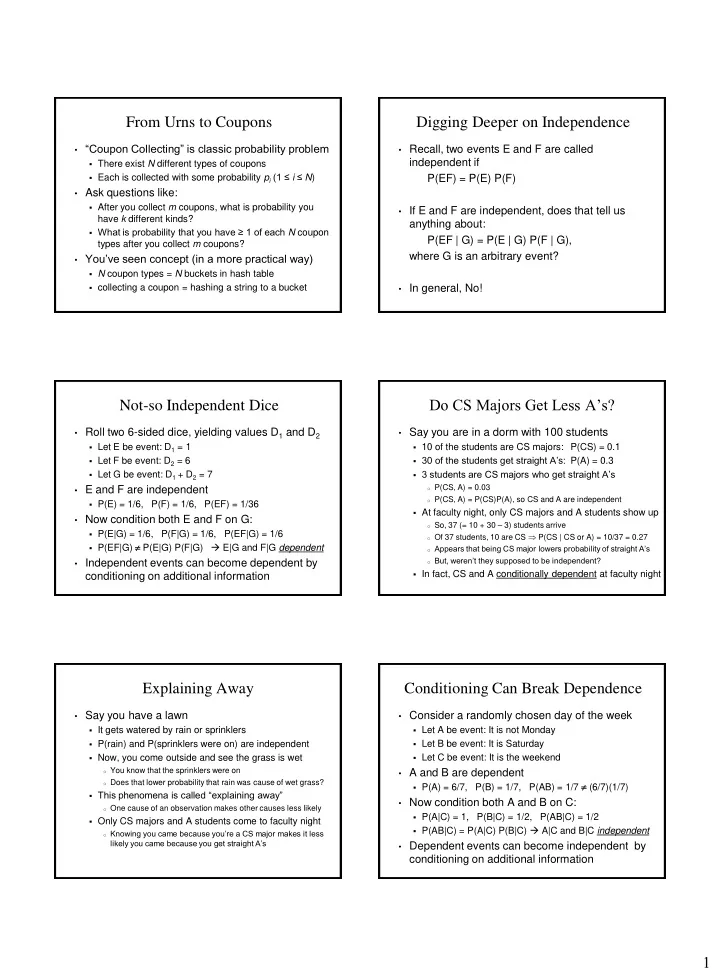
From Urns to Coupons Digging Deeper on Independence • “Coupon Collecting” is classic probability problem • Recall, two events E and F are called independent if  There exist N different types of coupons  Each is collected with some probability p i (1 ≤ i ≤ N ) P(EF) = P(E) P(F) • Ask questions like:  After you collect m coupons, what is probability you • If E and F are independent, does that tell us have k different kinds? anything about:  What is probability that you have ≥ 1 of each N coupon P(EF | G) = P(E | G) P(F | G), types after you collect m coupons? where G is an arbitrary event? • You’ve seen concept (in a more practical way)  N coupon types = N buckets in hash table  collecting a coupon = hashing a string to a bucket • In general, No! Do CS Majors Get Less A’s? Not-so Independent Dice • Roll two 6-sided dice, yielding values D 1 and D 2 • Say you are in a dorm with 100 students  Let E be event: D 1 = 1  10 of the students are CS majors: P(CS) = 0.1  30 of the students get straight A’s: P(A) = 0.3  Let F be event: D 2 = 6  3 students are CS majors who get straight A’s  Let G be event: D 1 + D 2 = 7 o P(CS, A) = 0.03 • E and F are independent o P(CS, A) = P(CS)P(A), so CS and A are independent  P(E) = 1/6, P(F) = 1/6, P(EF) = 1/36  At faculty night, only CS majors and A students show up • Now condition both E and F on G: o So, 37 (= 10 + 30 – 3) students arrive  P(E|G) = 1/6, P(F|G) = 1/6, P(EF|G) = 1/6 o Of 37 students, 10 are CS  P(CS | CS or A) = 10/37 = 0.27  P(EF|G)  P(E|G) P(F|G)  E|G and F|G dependent o Appears that being CS major lowers probability of straight A’s o But, weren’t they supposed to be independent? • Independent events can become dependent by  In fact, CS and A conditionally dependent at faculty night conditioning on additional information Explaining Away Conditioning Can Break Dependence • Say you have a lawn • Consider a randomly chosen day of the week  It gets watered by rain or sprinklers  Let A be event: It is not Monday  P(rain) and P(sprinklers were on) are independent  Let B be event: It is Saturday  Let C be event: It is the weekend  Now, you come outside and see the grass is wet o You know that the sprinklers were on • A and B are dependent o Does that lower probability that rain was cause of wet grass?  P(A) = 6/7, P(B) = 1/7, P(AB) = 1/7  (6/7)(1/7)  This phenomena is called “explaining away” • Now condition both A and B on C: o One cause of an observation makes other causes less likely  P(A|C) = 1, P(B|C) = 1/2, P(AB|C) = 1/2  Only CS majors and A students come to faculty night  P(AB|C) = P(A|C) P(B|C)  A|C and B|C independent o Knowing you came because you’re a CS major makes it less likely you came because you get straight A’s • Dependent events can become independent by conditioning on additional information 1

Conditional Independence Random Variable • Two events E and F are called conditionally • A Random Variable is a real-valued function independent given G , if defined on a sample space P(E F | G) = P(E | G) P(F | G) • Example:  3 fair coins are flipped. Or, equivalently: P(E | F G) = P(E | G)  Y = number of “heads” on 3 coins  Y is a random variable • Exploiting conditional independence to generate  P(Y = 0) = 1/8 (T, T, T) fast probabilistic computations is one of the main  P(Y = 1) = 3/8 (H, T, T), (T, H, T), (T, T, H) contributions CS has made to probability theory  P(Y = 2) = 3/8 (H, H, T), (H, T, H), (T, H, H)  P(Y = 3) = 1/8 (H, H, H)  P(Y ≥ 4) = 0 Binary Random Variables Simple Game • A binary random variable is a random variable • Urn has 11 balls (3 blue, 3 red, 5 black) with 2 possible outcomes  3 balls drawn. +$1 for blue, -$1 for red, $0 for black  n coin flips, each which independently come up heads  Y = total winnings with probability p           5 3 3 5 11 55              P(Y = 0) =            Y = number of “heads” on n flips  3   1   1   1   3  165   n               3 5 3 3 11 39 k n k  P(Y = k) = , where k = 0, 1, 2, ..., n   p ( 1 p )              P(Y = 1) =           = P(Y = -1)   k           1 2 2 1 3 165   n n        3 5 11 15      k n k         P(Y = 2) = = P(Y = -2)  So,   p ( 1 p ) 1        k   2   1   3  165  k 0       3 11 1 n n                 P(Y = 3) =     = P(Y = -3) k n k n n   p ( 1 p ) ( p ( 1 p )) 1 1  Proof:  3   3  165   k  k 0 Probability Mass Functions PMF For a Single 6-Sided Die • A random variable X is discrete if it has countably many values (e.g., x 1 , x 2 , x 3 , ...) 1/6 • Probability Mass Function (PMF) of a discrete p(x) random variable is:   p ( a ) P ( X a )    • Since , it follows that: p ( x ) 1 i  i 1    p ( x ) 0 for i 1 , 2 , ...    i P ( X a )   p ( x ) 0 otherwise X = outcome of roll where X can assume values x 1 , x 2 , x 3 , ... 2

PMF For a Roll of Two 6-Sided Dice Cumulative Distribution Functions • For a random variable X, the Cumulative 6/36 Distribution Function (CDF) is defined as: 5/36        F ( a ) F ( X a ) where a 4/36 p(x) 3/36 2/36 • The CDF of a discrete random variable is: 1/36     F ( a ) F ( X a ) p ( x )  all x a X = total rolled CDF For a Single 6-Sided Die Expected Value • The Expected Values for a discrete random 5/6 variable X is defined as: 4/6   E [ X ] x p ( x ) 3/6  p(x) x : p ( x ) 0 2/6 • Note: sum over all values of x that have p(x) > 0. 1/6 • Expected value also called: Mean , Expectation , Weighted Average , Center of Mass , 1 st Moment X = outcome of roll Expected Value Examples Indicator Variables • Roll a 6-Sided Die. X is outcome of roll • A variable I is called an indicator variable for event A if  p(1) = p(2) = p(3) = p(4) = p(5) = p(6) = 1/6              1 if occurs A 1 1 1 1 1 1 7                     • E[X] = 1 2 3 4 5 6 I             6 6 6 6 6 6 2  c 0 if A occurs • Y is random variable • What is E[ I ]?  P(Y = 1) = 1/3, P(Y = 2) = 1/6, P(Y = 3) = 1/2 p(0) = 1 – P(A)  p(1) = P(A), • E[Y] = 1 (1/3) + 2 (1/6) + 3 (1/2) = 13/6  E[ I ] = 1 P(A) + 0 (1 – P(A)) = P(A) 3

Lying With Statistics Lying With Statistics “There are three kinds of lies: “There are three kinds of lies: lies, damned lies, and statistics” lies, damned lies, and statistics” – Mark Twain – Mark Twain • School has 3 classes with 5, 10 and 150 students • School has 3 classes with 5, 10 and 150 students • Randomly choose a class with equal probability • Randomly choose a student with equal probability • X = size of chosen class • Y = size of class that student is in • What is E[X]? • What is E[Y]?  E[X] = 5 (1/3) + 10 (1/3) + 150 (1/3)  E[Y] = 5 (5/165) + 10 (10/165) + 150 (150/165) = 22635/165  137 = 165/3 = 55 • Note: E[Y] is students’ perception of class size  But E[X] is what is usually reported by schools! Expectation of a Random Variable Other Properties of Expectations • Let Y = g(X), where g is real-valued function • Linearity:    E [ aX b ] aE [ X ] b       E [ g ( X )] E [ Y ] y p ( y ) y p ( x ) j j j i  Consider X = 6-sided die roll, Y = 2X – 1.  i : g ( x ) y j j i j       g ( x ) p ( x ) g ( x ) p ( x )  E[X] = 3.5 E[Y] = 6 i i i i   i : g ( x ) y i : g ( x ) y j j i j i j   g ( x ) p ( x ) • N -th Moment of X: i i i   n n E [ X ] x p ( x )  x : p ( x ) 0  We’ll see the 2 nd moment soon... Utility • Utility is value of some choice  2 choices, each with n consequences: c 1 , c 2 ,..., c n  One of c i will occur with probability p i  Each consequence has some value (utility): U(c i )  Which choice do you make? • Example: Buy a $1 lottery ticket (for $1M prize)?  Probability of winning is 1/10 7  Buy : c 1 = win, c 2 = lose, U(c 1 ) = 10 6 – 1, U(c 2 ) = -1  Don’t Buy : c 1 = lose, U(c 1 ) = 0  E(buy) = 1/10 7 (10 6 – 1) + (1 – 1/10 7 ) (-1)  -0.9  E(don’t buy) = 1 (0) = 0  “You can’t lose if you don’t play!” 4