1 Multi-armed bandit problem A natural generalization Exponential - PDF document

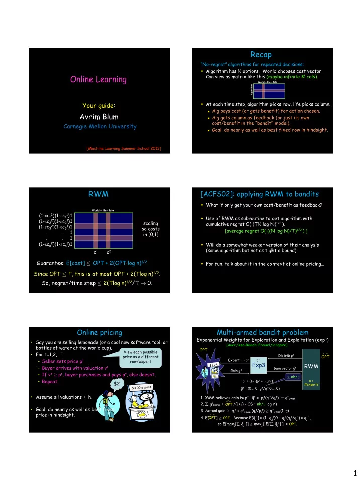
Recap “No - regret” algorithms for repeated decisions:  Algorithm has N options. World chooses cost vector. Online Learning Can view as matrix like this (maybe infinite # cols) World – life - fate Algorithm  At each time step, algorithm picks row, life picks column. Your guide:  Alg pays cost (or gets benefit) for action chosen. Avrim Blum  Alg gets column as feedback (or just its own cost/benefit in the “bandit” model). Carnegie Mellon University  Goal: do nearly as well as best fixed row in hindsight. [Machine Learning Summer School 2012] RWM [ACFS02]: applying RWM to bandits  What if only get your own cost/benefit as feedback? World – life - fate (1- e c 12 ) (1- e c 11 ) 1  Use of RWM as subroutine to get algorithm with (1- e c 2 2 ) (1- e c 2 1 ) 1 scaling cumulative regret O( (TN log N) 1/2 ). (1- e c 32 ) (1- e c 31 ) 1 so costs [average regret O( ((N log N)/T) 1/2 ).] . . 1 in [0,1] . . 1 (1- e c n2 ) (1- e c n1 ) 1  Will do a somewhat weaker version of their analysis (same algorithm but not as tight a bound). c 1 c 2 Guarantee: E[cost] · OPT + 2(OPT ¢ log n) 1/2  For fun, talk about it in the context of online pricing… Since OPT · T, this is at most OPT + 2(Tlog n) 1/2 . So, regret/time step · 2(Tlog n) 1/2 /T ! 0. Online pricing Multi-armed bandit problem Exponential Weights for Exploration and Exploitation (exp 3 ) • Say you are selling lemonade (or a cool new software tool, or [Auer,Cesa-Bianchi,Freund,Schapire] bottles of water at the world cup). OPT View each possible • For t=1,2 ,…T Distrib p t price as a different OPT Expert i ~ q t q t – Seller sets price p t row/expert Exp3 RWM – Buyer arrives with valuation v t Gain vector ĝ t Gain g it – If v t ¸ p t , buyer purchases and pays p t , else doesn’t. · nh/ ° – Repeat. q t = (1- ° )p t + ° unif n = $2 #experts ĝ t = (0,…,0, g it /q it ,0,…,0) • Assume all valuations · h. 1. RWM believes gain is: p t ¢ ĝ t = p it (g it /q it ) ´ g tRWM 2.  t g tRWM ¸ /(1+ ² ) - O( ² -1 nh/ ° log n) OPT • Goal: do nearly as well as best fixed 3. Actual gain is: g it = g tRWM (q it /p it ) ¸ g tRWM (1- ° ) price in hindsight. 4. E[ ] ¸ OPT . Because E[ĝ jt ] = (1- q jt )0 + q jt (g jt /q jt ) = g jt , OPT so E[max j [  t ĝ jt ]] ¸ max j [ E[  t ĝ jt ] ] = OPT. 1

Multi-armed bandit problem A natural generalization Exponential Weights for Exploration and Exploitation (exp 3 ) (Going back to full-info setting, thinking about paths…) [Auer,Cesa-Bianchi,Freund,Schapire]  A natural generalization of our regret goal is: what if we OPT also want that on rainy days, we do nearly as well as the Distrib p t OPT Expert i ~ q t q t best route for rainy days. Exp3 RWM  And on Mondays, do nearly as well as best route for Gain vector ĝ t Gain g it Mondays. · nh/ ° q t = (1- ° )p t + ° unif n =  More generally, have N “rules” (on Monday, use path P). #experts ĝ t = (0,…,0, g it /q it ,0,…,0) Goal: simultaneously, for each rule i, guarantee to do nearly as well as it on the time steps in which it fires.  For all i, want E[cost i (alg)] · (1+ e )cost i (i) + O( e -1 log N). Conclusion ( ° = ² ) : (cost i (X) = cost of X on time steps where rule i fires.) E[Exp3] ¸ OPT/(1+ ² ) 2 - O( ² -2 nh log(n))  Can we get this? Balancing would give O((OPT nh log n) 2/3 ) in bound because of ² -2 . But can reduce to ² -1 and O((OPT nh log n) 1/2 ) more care in analysis. A natural generalization A simple algorithm and analysis (all on one slide)  Start with all rules at weight 1.  This generalization is esp natural in machine learning for combining multiple if-then rules.  At each time step, of the rules i that fire,  E.g., document classification. Rule: “if <word -X> appears select one with probability p i / w i . then predict <Y>”. E.g., if has football then classify as  Update weights: sports.  If didn’t fire, leave weight alone.  So, if 90% of documents with football are about sports,  If did fire, raise or lower depending on performance we should have error · 11% on them. compared to weighted average: “Specialists” or “sleeping experts” problem.  r i = [  j p j cost(j)]/(1+ e ) – cost(i)  w i à w i (1+ e ) ri  So, if rule i does exactly as well as weighted average, its weight drops a little. Weight increases if does  Assume we have N rules, explicitly given. better than weighted average by more than a (1+ e ) factor. This ensures sum of weights doesn’t increase.  For all i, want E[cost i (alg)] · (1+ e )cost i (i) + O( e -1 log N).  Final w i = (1+ e ) E[costi(alg)]/(1+ e )-costi(i) . So, exponent · e -1 log N. (cost i (X) = cost of X on time steps where rule i fires.)  So, E[cost i (alg)] · (1+ e )cost i (i) + O( e -1 log N). Lots of uses Adapting to change  Can combine multiple if-then rules  What if we want to adapt to change - do nearly as well as best recent expert?  Can combine multiple learning algorithms:  For each expert, instantiate copy who wakes up on day t  Back to driving, say we are given N “conditions” to pay for each 0 · t · T-1. attention to (is it raining?, is it a Monday?, …).  Our cost in previous t days is at most (1+ ² )(best expert in last t days) + O( ² -1 log(NT)).  Create N rules: “ if day satisfies condition i, then use  (not best possible bound since extra log(T) but not bad). output of Alg i ”, where Alg i is an instantiation of an experts algorithm you run on just the days satisfying that condition .  Simultaneously, for each condition i, do nearly as well as Alg i which itself does nearly as well as best path for condition i. 2

More general forms of regret Summary Algorithms for online decision-making with 1. “best expert” or “external” regret: strong guarantees on performance compared – Given n strategies. Compete with best of them in hindsight. to best fixed choice. 2. “sleeping expert” or “regret with time - intervals”: Application: play repeated game against • – Given n strategies, k properties. Let S i be set of days adversary. Perform nearly as well as fixed satisfying property i (might overlap). Want to strategy in hindsight. simultaneously achieve low regret over each S i . Can apply even with very limited feedback. 3. “internal” or “swap” regret: like (2), except that S i = set of days in which we chose strategy i. Application: which way to drive to work, with • only feedback about your own paths; online pricing, even if only have buy/no buy feedback. Internal/swap-regret Weird… why care? “Correlated equilibrium” • E.g., each day we pick one stock to buy • Distribution over entries in matrix, such that if a shares in. trusted party chooses one at random and tells – Don’t want to have regret of the form “every you your part, you have no incentive to deviate. time I bought IBM, I should have bought R P S • E.g., Shapley game. Microsoft instead”. • Formally, regret is wrt optimal function -1,-1 -1,1 1,-1 R f:{1,…,n} ! {1,…,n} such that every time you P 1,-1 -1,-1 -1,1 played action j, it plays f(j). -1,1 1,-1 -1,-1 S In general-sum games, if all players have low swap- regret, then empirical distribution of play is apx correlated equilibrium. Can convert any “best expert” algorithm A into one Internal/swap-regret, contd achieving low swap regret. Idea: Algorithms for achieving low regret of this – Instantiate one copy A j responsible for expected regret over times we play j. form: A 1 – Foster & Vohra, Hart & Mas-Colell, Fudenberg Q Play p = pQ & Levine. Alg q 2 A 2 – Will present method of [BM05] showing how to Cost vector c p 2 c convert any “best expert” algorithm into one . . . achieving low swap regret. A n – Allows us to view p j as prob we play action j, or as prob we play alg A j . – Give A j feedback of p j c. – A j guarantees  t (p j t c t ) ¢ q j t · min i  t p j t c i t + [regret term] – Write as:  t p j t (q j t ¢ c t ) · min i  t p j t c i t + [regret term] 3