1 s Markov Decision Processes Graphical View of MDP a s, a - PDF document
Logistics 1 HW 1 Monte Monte- -Carlo Planning: Carlo Planning: Basic Principles and Recent Progress Basic Principles and Recent Progress Dan Weld UW CSE 573 October 2012 Most slides by Alan Fern Consistency &
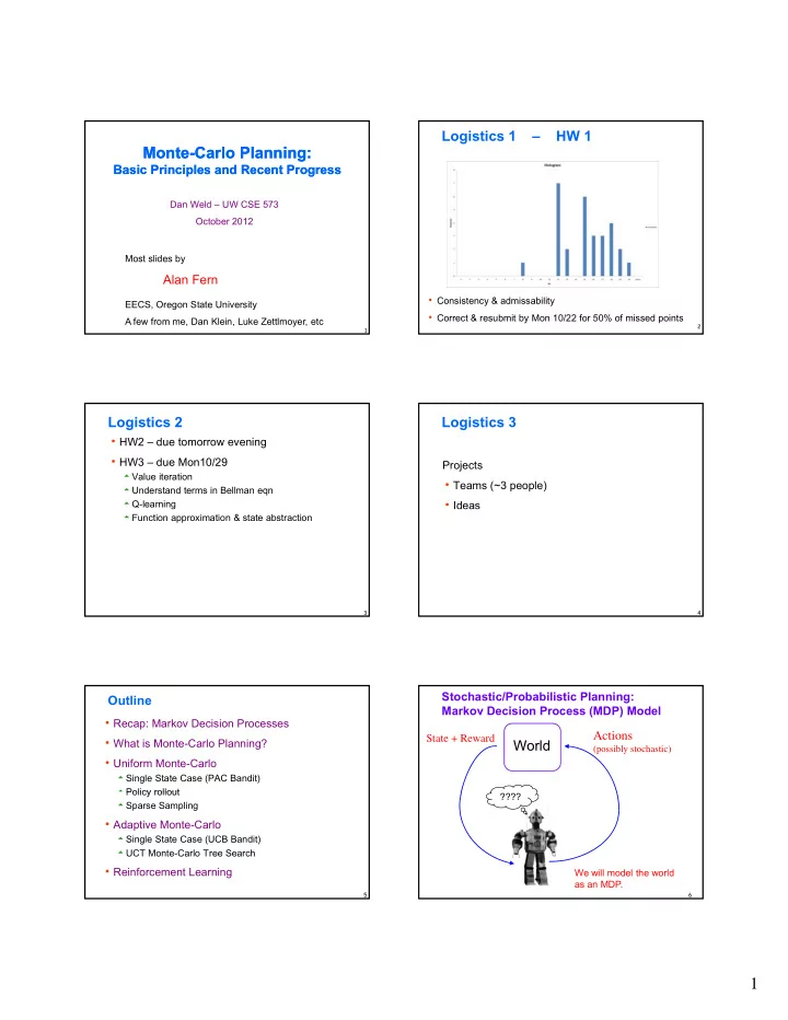
Logistics 1 – HW 1 Monte Monte- -Carlo Planning: Carlo Planning: Basic Principles and Recent Progress Basic Principles and Recent Progress Dan Weld – UW CSE 573 October 2012 Most slides by Alan Fern Consistency & admissability EECS, Oregon State University Correct & resubmit by Mon 10/22 for 50% of missed points A few from me, Dan Klein, Luke Zettlmoyer, etc 2 1 Logistics 2 Logistics 3 HW2 – due tomorrow evening HW3 – due Mon10/29 Projects Value iteration Teams (~3 people) Understand terms in Bellman eqn Q-learning Ideas Function approximation & state abstraction 3 4 Stochastic/Probabilistic Planning: Outline Markov Decision Process (MDP) Model Recap: Markov Decision Processes Actions State + Reward What is Monte-Carlo Planning? World (possibly stochastic) Uniform Monte-Carlo Single State Case (PAC Bandit) Policy rollout Policy rollout ???? Sparse Sampling Adaptive Monte-Carlo Single State Case (UCB Bandit) UCT Monte-Carlo Tree Search Reinforcement Learning We will model the world as an MDP. 5 6 1
s Markov Decision Processes Graphical View of MDP a s, a s,a,s’ s’ S t S t+1 S t+2 $R A t A t+1 A t+2 An MDP has four components: S, A, P R , P T : finite state set S R t R t R t+1 R R t+2 R t 2 1 finite action set A Transition distribution P T (s’ | s, a) Probability of going to state s’ after taking action a in state s First-Order Markovian dynamics (history independence) Next state only depends on current state and current action First-order Markov model Bounded reward distribution P R (r | s, a) First-Order Markovian reward process Probability of receiving immediate reward r after exec a in s Reward only depends on current state and action First-order Markov model 7 8 Policies (“plans” for MDPs) Recap: Defining MDPs Given an MDP we wish to compute a policy Policy, Could be computed offline or online. Function that chooses an action for each state A policy is a possibly stochastic mapping from states to actions Value function of policy π: S → A Aka Utility π (s) is action to do at state s ( ) Sum of discounted rewards from following policy S f di t d d f f ll i li π (s) specifies a continuously reactive controller Objective? Find policy which maximizes expected utility, V(s) How to measure goodness of a policy? 10 Value Function of a Policy Relation to Infinite Horizon Setting We consider finite-horizon discounted reward, Often value function V π (s) is defined over infinite discount factor 0 ≤ β < 1 horizons for a discount factor 0 ≤ β < 1 V π (s,h) denotes expected h-horizon discounted total t t V ( s ) E [ R | , s ] reward of policy π at state s 0 t Each run of π for h steps produces a random reward It is easy to show that difference between V (s h) and It is easy to show that difference between V π (s,h) and sequence: R 1 R 2 R 3 … R h R R R R V π (s) shrinks exponentially fast as h grows V π (s,h) is the expected discounted sum of this sequence h R t V ( s , h ) E R | , s h ( ) ( , ) max V s V s h t 1 0 t Optimal policy π * is policy that achieves maximum h-horizon results apply to infinite horizon setting value across all states 11 12 2
Computing the Best Policy Bellman Equations for MDPs Optimal policy maximizes value at each state (1920 ‐ 1984) Q*(a, s) Optimal policies guaranteed to exist [Howard, 1960] When state and action spaces are small and MDP is known we find optimal policy in poly-time p p y p y With value iteration Or policy Iteration Both use…? 14 Bellman Backup Computing the Best Policy V i+1 V i What if… Space is exponentially large? s 1 MDP transition & reward models are unknown? a 1 V 0 = 0 V 1 = 6.5 5 s 0 a 2 s 2 V 0 = 1 a 3 s 3 V 0 = 2 max 16 Large Worlds: Monte-Carlo Approach Large Worlds: Model-Based Approach Often a simulator of a planning domain is available 1. Define a language for compactly describing MDP or can be learned from data model, for example: Even when domain can’t be expressed via MDP language Dynamic Bayesian Networks Probabilistic STRIPS/PDDL Fire & Emergency Response g y p 2. Design a planning algorithm for that language D i l i l i h f h l Klondike Solitaire Problem: more often than not, the selected language is inadequate for a particular problem, e.g. Problem size blows up Fundamental representational shortcoming 17 18 18 3
Large Worlds: Monte-Carlo Approach Example Domains with Simulators Traffic simulators Robotics simulators Monte-Carlo Planning: compute a good policy for Military campaign simulators an MDP by interacting with an MDP simulator Computer network simulators Emergency planning simulators large-scale disaster and municipal action World Sports domains (Madden Football) Simulator Real Board games / Video games World Go / RTS State + reward In many cases Monte-Carlo techniques yield state-of-the-art performance. Even in domains where model-based planner is applicable. 19 19 20 MDP: Simulation-Based Representation Slot Machines as MDP? A simulation-based representation gives: S, A, R, T: finite state set S (generally very large) finite action set A Stochastic, real-valued, bounded reward function R(s,a) = r … Stochastically returns a reward r given input s and a Can be implemented in arbitrary programming language Can be implemented in arbitrary programming language ???? Stochastic transition function T(s,a) = s’ (i.e. a simulator) Stochastically returns a state s’ given input s and a Probability of returning s’ is dictated by Pr(s’ | s,a) of MDP T can be implemented in an arbitrary programming language 21 22 Single State Monte-Carlo Planning Outline Suppose MDP has a single state and k actions Preliminaries: Markov Decision Processes Figure out which action has best expected reward What is Monte-Carlo Planning? Can sample rewards of actions using calls to simulator Sampling a is like pulling slot machine arm with random Uniform Monte-Carlo payoff function R(s,a) Single State Case (Uniform Bandit) s Policy rollout Policy rollout a k a 1 a 2 Sparse Sampling Adaptive Monte-Carlo … Single State Case (UCB Bandit) UCT Monte-Carlo Tree Search … R(s,a 2 ) R(s,a k ) R(s,a 1 ) Multi-Armed Bandit Problem 23 24 4
UniformBandit Algorithm PAC Bandit Objective NaiveBandit from [Even-Dar et. al., 2002] Probably Approximately Correct (PAC) 1. Pull each arm w times (uniform pulling). Select an arm that probably (w/ high probability, 1- ) has approximately (i.e., within ) the best expected reward 2. Return arm with best average reward. s Use as few simulator calls (or pulls) as possible s a 1 a 2 a k a 1 a 2 a k … … r 11 r 12 … r 1w r 21 r 22 … r 2w … r k1 r k2 … r kw … R(s,a 1 ) R(s,a 2 ) R(s,a k ) How large must w be to provide a PAC guarantee? Multi-Armed Bandit Problem 25 26 UniformBandit Algorithm Aside: Additive Chernoff Bound NaiveBandit from [Even-Dar et. al., 2002] • Let R be a random variable with maximum absolute value Z. An let r i (for i=1,…,w) be i.i.d. samples of R 1. Pull each arm w times (uniform pulling). • The Chernoff bound gives a bound on the probability that the 2. Return arm with best average reward. average of the r i are far from E[R] s 2 w Chernoff a 1 a 2 a k 1 Pr E [ [ R ] ] r exp p w B Bound d w i i Z i 1 … Equivalently: With probability at least we have that, 1 r 11 r 12 … r 1w r 21 r 22 … r 2w … r k1 r k2 … r kw w [ ] 1 1 ln 1 E R r Z w i w How large must w be to provide a PAC guarantee? 1 i 27 28 UniformBandit PAC Bound # Simulator Calls for UniformBandit s With a bit of algebra and Chernoff bound we get: a 1 a 2 a k 2 R max If for all arms simultaneously w ln k w … [ ( , )] 1 E R s a r i ij w j 1 … R(s,a k ) with probability at least R(s,a 1 ) R(s,a 2 ) 1 k That is, estimates of all actions are ε –accurate with Total simulator calls for PAC: k w O ln k 2 probability at least 1- Thus selecting estimate with highest value is Can get rid of ln(k) term with more complex approximately optimal with high probability, or PAC algorithm [Even-Dar et. al., 2002]. 29 30 5
Recommend
More recommend
Explore More Topics
Stay informed with curated content and fresh updates.



![DCS/CSCI 2350: Social & Economic Networks Sponsored Search Market Reading: Chapter 15 [EK]](https://c.sambuz.com/768025/dcs-csci-2350-social-economic-networks-s.webp)
