1 Estimation from outbreaks when R 0 < 1 Estimating R 0 : from - PDF document
Outline Parameter estimation, uncertainty, Estimating R 0 model fitting, model selection, Parameter estimation - Likelihood approaches and sensitivity and uncertainty analysis - Bayesian approaches Fitting more complex models Jamie
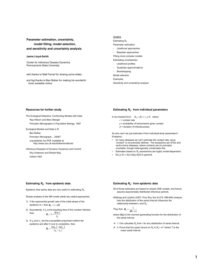
Outline Parameter estimation, uncertainty, Estimating R 0 model fitting, model selection, Parameter estimation - Likelihood approaches and sensitivity and uncertainty analysis - Bayesian approaches Fitting more complex models Jamie Lloyd-Smith Estimating uncertainties Center for Infectious Disease Dynamics - Likelihood profiles Pennsylvania State University - Quadratic approximations - Bootstrapping with thanks to Matt Ferrari for sharing some slides, Model selection Examples and big thanks to Ben Bolker for making his wonderful book available online. Sensitivity and uncertainty analysis Resources for further study Estimating R 0 : from individual parameters The Ecological Detective: Confronting Models with Data R 0 = β / γ = c p D where In its simplest form, Ray Hilborn and Marc Mangel c = contact rate Princeton Monographs in Population Biology, 1997 p = probability of transmission given contact D = duration of infectiousness Ecological Models and Data in R Ben Bolker So why can’t we just estimate it from individual-level parameters? Problems: Princeton Monograph… 2008? • for many diseases we can’t estimate the contact rate, since unpublished, but PDF available at “contact” is not precisely defined. The exceptions are STDs and http://www.zoo.ufl.edu/bolker/emdbook/ vector-borne diseases, where contacts are (in principle) countable, though heterogeneity complicates this. Infectious Diseases of Humans: Dynamics and Control • Estimates based on R 0 expressions are highly model-dependent. Roy Anderson and Robert May • E( c p D ) ∫ E( c ) E( p ) E( D ) in general. Oxford 1991 Estimating R 0 : from epidemic data Estimating R 0 : from epidemic data All of those estimates are based on simple ODE models, and hence Epidemic time series data are very useful in estimating R 0 . assume exponentially distributed infectious periods. Simple analysis of the SIR model yields two useful approaches: Wallinga and Lipsitch (2007, Proc Roy Soc B 274: 599-604) analyze how the distribution of the serial interval influences the 1) If the exponential growth rate of the initial phase of the relationship between r and R 0 . epidemic is r , then = 1 + R rD 0 1 = They find R 2) Equivalently, if t d is the doubling time of the number infected, 0 − M ( r ) then D ln 2 = + R 1 where M ( z ) is the moment generating function for the distribution of 0 t d the serial interval. 3) If s 0 and s ∝ are the susceptible proportions before the � 1. Can calculate R 0 from r for any distribution of serial interval. epidemic and after it runs to completion, then ( ) ( ) − � 2. Prove that the upper bound on R 0 is R 0 = e rT where T is the ln s ln s = ∞ 0 R − 0 mean serial interval. ( s s ) ∞ 0 1
Estimation from outbreaks when R 0 < 1 Estimating R 0 : from epidemic data If case data are collected in discrete intervals, estimation from Measles outbreaks in continuous-time models is difficult. vaccinated populations, UK Ferrari et al (2005, Math Biosci 198: 14-26) derive an approach based on chain binomial models that provides a maximum- likelihood estimator for R 0 and the associated uncertainty. Posterior distribution Outbreak size on R eff under two models Branching process models allow analysis of outbreak size to make inference about the effective reproductive number when R eff <1. But, like the s ∝ approaches, it requires that the epidemic runs to its natural completion. Farrington et al (2003) Biostatistics 4: 279-295. Estimating R 0 : from endemic data Estimating R 0 : from endemic data Anderson & May derive a number of simple expressions for Anderson & May derive a number of simple expressions for R 0 in R 0 in the endemic setting. the endemic setting. Their results depend on the age-dependent rate of mortality R ≈ For Type I mortality, L A in the population μ ( a ), which yields a “Type I” or “Type II” 0 mortality curve. where L is the mean lifespan and A is the mean age at first infection. R = For Type II mortality, exactly. L A 0 Of course, these simple estimates depend on strong assumptions Type I about random mixing, no heterogeneities, no age-dependence of the force of infection, and constant population size. Type II See later chapters of Anderson & May, or Dietz (1993) Stat Meth Med Res 2: 23-41, for more advanced treatments. Estimating R 0 : from age-seroprevalence data From age-seroprevalence data, the age-dependent force of infection can be estimated directly. To estimate R 0 , need to make assumption about WAIFW matrix. And see comprehensive review: “Estimation of the basic reproductive number for infectious diseases from age-stratified serological survey data” (2001) Appl Statist 50: 251-292. 2
Fitting single distributions: method of moments Fitting single distributions A fancy name for a simple idea: Observed offspring distribution for Observed distribution of For most standard probability distributions, the parameters SARS in Singapore incubation periods for SARS can be expressed in terms of the moments of the distribution (e.g. the mean and variance). e.g. exponential distribution, f ( x ) = λ exp(- λ x ) λ = 1/ μ Method of moments: calculate the sample moments from your data, and plug them into these expressions λ ≈ μ 1 t 4 6 8 10 12 Estimates may be biased, but this is a good way to get a quick days estimate. Fitting single distributions: maximum likelihood Example: the binomial distribution The binomial distribution describes the number of successes The likelihood is the probability of observing the data given the out of N trials, if each trial has probability p of success. model (and parameter values for the model). For a single observation from a binomial distribution (say, the number of susceptibles infected in a day, out of a beginning Y = data set, {Y 1 , Y 2 , … Y n } total of N), the likelihood that k out of N are infected, if the p = model parameters per capita infection probability is p, is Then the likelihood is Λ = Pr(Y|p), where the “model” (in this case the probability distribution If we have n independent observations of this process, each we’re fitting) will determine the form of the probability. with the same number of susceptibles N, and the number infected on the i th observation is k i , then the likelihood is The basic idea of maximum likelihood estimation (MLE) is to find the parameter set that maximizes the likelihood of observing your data. Likelihood example: binomial distribution Likelihood example: binomial distribution We now want to find the parameter p that maximizes L . For this simple example, it can actually be calculated analytically, and yields a sensible answer: It is conventional to work with the log-likelihood, L = log( � ), for two reasons: (1) It turns the product (which arises from the joint probability of many independent observations) into a sum. (2) The probabilities are often very small numbers (usually <<1!), and working with a product of small numbers Example plot of causes numerical problems in computation. binomial likelihood The log-likelihood for our binomial problem is: curve and fit to data, from Bolker 200X. probability p 3
Recommend
More recommend
Explore More Topics
Stay informed with curated content and fresh updates.


