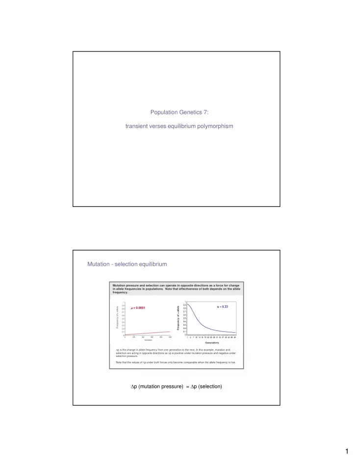

Population Genetics 7: transient verses equilibrium polymorphism Mutation - selection equilibrium Mutation pressure and selection can operate in opposite directions as a force for change in allele frequencies in populations. Note that effectiveness of both depends on the allele frequency. Frequency of a allele µ = 0.0001 ∆ p is the change in allele frequency from one generation to the next. In this example, mutation and selection are acting in opposite directions as ∆ p is positive under mutation pressure and negative under selection pressure. Note that the values of ∆ p under both forces only become comparable when the allele frequency is low. ∆ p (mutation pressure) = ∆ p (selection) 1
Mutation - selection equilibrium 1. Mutation pressure: ( ) ( ) ∆ = µ − Let µ = the mutation rate from A ⇒ a q p q v { { The freq of A alleles Let ν = the mutation rate from a ⇒ A The freq of a alleles that change to a by that change to A by µ ν mutaion at rate mutation at rate Let p t = the frequency of A in the population in generation t . Let q t = the frequency of a in the population in generation t , with q t = (1 – p t ). 2. Natural selection against a deleterious recessive allele: So for ∆ q, Remember form our earlier lecture: ∆ q = qt +1 – qt qt +1 = qt - sqt 2 / 1- sq t 2 ∆ q = ( qt - sqt 2 / 1- sq t 2 ) – qt ∆ q = - sqt 2 (1- q ) / 1- sq t 2 Mutation - selection equilibrium ∆ q (mutation pressure) = ∆ q (selection) p µ - q ν = sqt 2 (1- q ) / 1- sq t 2 YUCK! [Approximate and simplify] p µ = sqt 2 (1- q) / 1- sqt 2 p µ = sqt 2 (1- q) (1-q) µ = sqt 2 (1- q) µ = sqt 2 (approx.) [Dominance: q = µ /hs (approx.)] 2
Mutation - selection equilibrium Attainment of the equilibrium allele frequency given selection and a variety of different mutation rates. Note that the time to equilibrium varies in addition to the actual equilibrium frequencies. s = 0.1 ( W aa = 0.9) µ = mut rate A → a a µ = 0.01 µ = 0.001 µ = 0.0001 µ = 0.00001 Note that fore realistic mutation rates, the equilibrium frequencies are quite low (freq of a allele > 0.05). In this example selection pressure is also quite weak ( s = 0.1). If we assume stronger selection pressure ( s > 0.1), the equilibrium point will be lower and the rate to equilibrium will be faster. Mutation - selection equilibrium Effect of partial dominance on mutation-selection equilibrium. The fitness of genotypes AA, Aa, and aa are assumed to be 1, 1–hs, and 1- s respectively. Equilibrium frequency of recessive allele ( a ) 0.035 0.03 h = 0 0.025 h = 0.01 h = 0.05 0.02 h = 0.1 h = 0.5 0.015 0.01 0.005 0 0.001 0.0001 0.00001 0.000001 Ratio of mutation rate to selection coefficient against aa ( µ /s) The symbol h is the amount of dominance in the heterozygote genotype. Note, that even a small amount of dominance (h = 0.01) reduced the equilibrium frequency of the recessive allele. Hence, dominance has a significant influence on the equilibrium point. The reason is that when q, the freq of the recessive allele is small, the majority of those alleles are in the heterozygote configuration, and even a small amount of selection on the heterozygotes leads to a major reduction in its equilibrium frequency as compared with full dominance. Note that for reasonable values of µ , h, and s, the equilibrium frequencies are < 0.01, This means that mutation selection equilibrium is not sufficient to explain low frequency detrimental alleles in populations where those alleles have frequencies > 0.01 3
Selection - drift equilibrium Drift alone: probability of fixation = 1/2N e Selection + Drift: probability of fixation depends on interaction of s and N e . N e s > 1 : beneficial allele more likely to be fixed than under drift alone N e s < 1 : beneficial allele is fixed with probability close to its frequency in the population Selection - drift Then fate of a beneficial recessive allele (A1) is not always predictable under the combined effects of directional selection and genetic drift. If there is no genetic drift (left: N e s = infinity), the fate of the recessive allele (A1) is always determined by selection. When there is drift (right: N e s < infinity) the fate of the recessive allele (A1) is not necessarily determined by selection; hence a deleterious allele can be fixed in a population. N e s = 100 N e s = infinity Note that N e s > 1 does not guarantee that an allele is going to be fixed, it simply indicates that (as a long term average) the frequency that it is fixed will be greater than the frequency under genetic drift alone. 4
Selection - drift equilibrium System Initial frequency Fixation N e s s Drift alone 100 1 0.01 1% Selection + Drift 100 0.1 0.01 10% Selection alone infinity 0.1 0.01 100% Selection - drift s 1 = 0.1 s 2 = 0.3 5
Selection - drift Equilibrium frequencies under balancing selection (s 1 = 0.1 and s 2 = 0.3) are less stable under the influence of genetic drift (right) as compared with an otherwise ideal population (left). Because drift disturbs the allele frequencies each generation, frequencies in any one generation will not be in equilibrium. However, the long term average will be the equilibrium frequencies. The polymorphism in both of the above cases is not transient. Selection - drift Polymorphisms under balancing selection ( s 1 = 0.1 and s 2 = 0.3) is transient if drift effects are strong. (N e = 50). 6
Mutation – selection – drift Combined effects of mutation, selection and drift on polymorphism. When drift is weak polymorphism is not transient, but when drift is strong the polymorphism is transient, but recurring due to mutation. N e s = 1000 N e s = infinity equilibrium N e s = 100 N e s = 10 Mutation – selection – drift Very high mutation rate (0.01) results in only a small shift in the long term average allele frequency under overdominant selection drift + mutation + selection µ = 0.01 drift + selection N e s = 1000 7
Mutation - drift equilibrium • Ignored until 1960’s • “ Neutral theory of molecular evolution” • Transient polymorphism • Fundamental to discipline of molecular evolution Sources of polymorphism in populations • Mutation-selection-drift equilibrium (long-term or transient) • Selection-drift (transient) • Overdominance-drift equilibrium (long-term or transient) • Mutation-drift (transient, but important) 8
Sources of polymorphism in populations • Drift constantly disturbs equilibrium. • The strength of the disturbance depends on the effective population size (N e ). • If strong enough, the disturbances can push the frequency to fixation. • We don’t expect to see persistent equilibrium in populations with low N e . • For realistic values of µ , h and s, the equilibrium point is generally very low ( p < 0.01). • As an explanation for natural polymorphisms > 0.01, the balance between mutation and selection is not satisfactory. • Overdominance can explain population polymorphisms with frequencies > 0.01. • A cost in fitness makes it unlikely that it can be invoked as a common mechanism in natural populations. • We will return the notion of the cost of selection later in this course. 9
Recommend
More recommend