1. Modelling Issues Modelling is more an art than a science! Choice - PowerPoint PPT Presentation

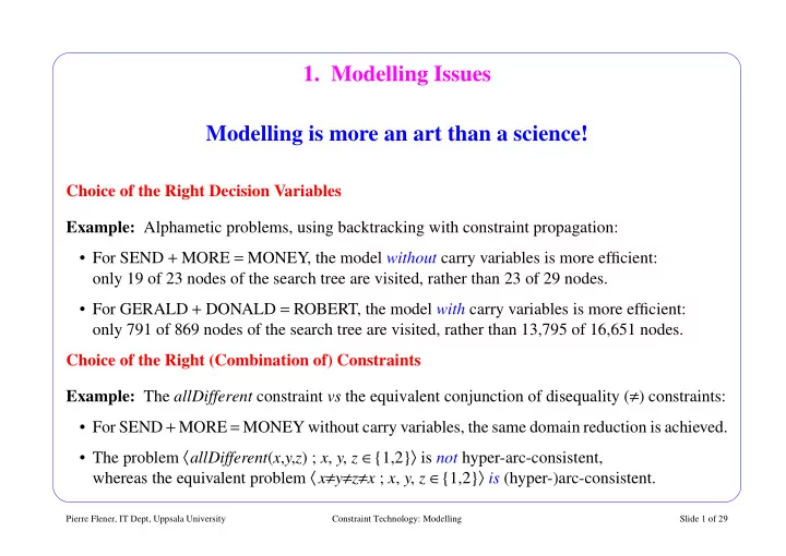
1. Modelling Issues Modelling is more an art than a science! Choice of the Right Decision Variables Example: Alphametic problems, using backtracking with constraint propagation: • For SEND + MORE = MONEY, the model without carry variables is more efficient: only 19 of 23 nodes of the search tree are visited, rather than 23 of 29 nodes. • For GERALD + DONALD = ROBERT, the model with carry variables is more efficient: only 791 of 869 nodes of the search tree are visited, rather than 13,795 of 16,651 nodes. Choice of the Right (Combination of) Constraints Example: The allDifferent constraint vs the equivalent conjunction of disequality ( ≠ ) constraints: • For SEND + MORE = MONEY without carry variables, the same domain reduction is achieved. • The problem 〈 allDifferent ( x , y , z ) ; x , y , z ∈ {1,2} 〉 is not hyper-arc-consistent, whereas the equivalent problem 〈 x ≠ y ≠ z ≠ x ; x , y , z ∈ {1,2} 〉 is (hyper-)arc-consistent. Pierre Flener, IT Dept, Uppsala University Constraint Technology: Modelling Slide 1 of 29

Choice of the Right Search Procedure • Consider using a computationally more expensive dynamic variable-and-value ordering , which takes into account the current state of the solver. • Use the first-fail principle to delay choice as long as possible: To succeed, try first where you are most likely to fail. For instance, select the decision variable with the smallest current domain. Optionally break ties by selecting the decision variable that appears in the largest number of currently active constraints. • Consider selecting first a value, and then a variable whose current domain contains that value. Rules of Thumb • The size of the search tree is a good measure of the complexity of the model. • Use few decision variables . • Use simple constraints with good solvers, especially global constraints . • Deploy constraint propagation techniques that require little preprocessing . • Avoid disjunctive constraints , as they often lead to large search trees. Careful: These rules of thumb (of course) have their exceptions: It is important to empirically test several combinations of models and search procedures. Pierre Flener, IT Dept, Uppsala University Constraint Technology: Modelling Slide 2 of 29

2. Reified Constraints Definition: The reified constraint (or reification ) of a primitive constraint c is the constraint c ⇔ B where B is a fresh Boolean decision variable, with truth represented by 1, and falsity by 0. Benefit: Possibly improved constraint propagation, when there are constraints on the introduced Boolean decision variables: • When the constraint c becomes satisfied (violated), its Boolean variable B can be set to 1 (0). • When the Boolean variable B is set to 1 (0), the constraint c ( ¬ c ) is added. Benefit: Reified constraints are also useful for expressing cardinality (or multiplicity ) constraints without recourse to disjunction. Example: Constraining two or three out of five given constraints c i to hold: c 1 ⇔ B 1 , c 2 ⇔ B 2 , c 3 ⇔ B 3 , c 4 ⇔ B 4 , c 5 ⇔ B 5 , 2 ≤ B 1 + B 2 + B 3 + B 4 + B 5 ≤ 3 Example: See the implementation of soft constraints in Section 8 (on slide 28). Careful: Not all primitive constraints are reifiable. Pierre Flener, IT Dept, Uppsala University Constraint Technology: Modelling Slide 3 of 29

3. Higher-Order Constraints Definition: A higher-order term is an integer term referring to the truth of a constraint, where truth is represented by 1, and falsity by 0. Notation: We here wrap the embedded constraint into parentheses. ∈ ∑ Example: The higher-order term ( [ ] ) Series j i = denotes the number of elements j Range of the array Series , which is indexed by the set Range , that are equal to a given element i . Benefit: A higher-order term represents an implicit reification. Definition: A higher-order constraint is a constraint involving higher-order terms. Benefit: Higher-order constraints are useful for expressing cardinality / multiplicity constraints . Example: See the two models of the Warehouse Location problem in Section 5 (on slide 7 and 8). Example: See the model for the Magic Series problem in Section 6 (on slide 13). Pierre Flener, IT Dept, Uppsala University Constraint Technology: Modelling Slide 4 of 29

4. Redundant Decision Variables and Channelling Constraints Definition: A redundant decision variable is a decision variable that represents information that is already represented by some other decision variable(s). Benefit: Some constraints may be easier to formulate, or may propagate better. Example: The reification of a constraint implicitly introduces a redundant decision variable. Definition: A channelling constraint is a constraint between mutually redundant decision variables establishing the consistency of their information. Benefit: Not all the decision variables need to be explicitly labelled during search. Example: The reification c ⇔ B channels between the decision variables of the constraint c and the Boolean decision variable B . Example: See the first model of the Warehouse Location problem in Section 5 (on slide 7). Example: See the redundant modelling of relation decision variables in Section 5 (on slide 11). Pierre Flener, IT Dept, Uppsala University Constraint Technology: Modelling Slide 5 of 29

5. Matrix Modelling and Relational Modelling Example: The Warehouse Location Problem A company considers opening warehouses on some candidate locations in order to supply its existing stores: • Each candidate warehouse has the same maintenance cost. • Each candidate warehouse has a supply capacity (the maximum number of stores it can supply). • The supply cost to a store depends on the warehouse. The objective is to determine which warehouses to open, and which of them should supply the various stores, subject to the following constraints : • Each store must be supplied by exactly one opened warehouse. • Each opened warehouse supplies at most a number of stores equal to its capacity. and cost function : • The sum of the actually incurred maintenance costs and supply costs is minimised. Pierre Flener, IT Dept, Uppsala University Constraint Technology: Modelling Slide 6 of 29

A First Matrix Model of the Warehouse Location Problem ( wlocation.prj ) Capacity: Berlin London Madrid Paris Rome 1 4 2 1 3 (instance data) SupplyCost: Berlin London Madrid Paris Rome 20 24 11 25 30 Store 1 … … … … … … Supply: Store 1 Store 2 … Store 10 ∈ Whs ∈ Whs ∈ Whs (decision variable) … OpenWhs ( ⊆ Whs ): Berlin London Madrid Paris Rome ∈ {0,1} ∈ {0,1} ∈ {0,1} ∈ {0,1} ∈ {0,1} ( redundant variables ) ∈ ∑ ∑ ⋅ minimise SupplyCost[s,Supply[s]] OpenWhs[w] MaintCost + ∈ s Stores w Whs ∀ ∈ ⋅ subject to s Stores OpenWhs[Supply[s]] ( channelling constraint ) = 1 ∈ ∑ ∀ ∈ ⋅ ≤ and w Whs (Supply[s]=w) Capacity[w] s Stores Pierre Flener, IT Dept, Uppsala University Constraint Technology: Modelling Slide 7 of 29

A Second Matrix Model of the Warehouse Location Problem ( wlocation2.prj ) Drop the matrix OpenWhs of redundant decision variables as well as the channelling constraint, and reformulate the second term of the cost function as the following third-order term:   ∑ ∈ ∑ ( ) > ⋅ Supply[s]=w MaintCost 0   w ∈ Whs s Stores This model is an order of magnitude more efficient, in OPL on the considered instance data. Redundancy elimination may pay off, but it may just as well be the converse. But this is hard to guess, as human intuition may be weak here. Disadvantages of OPL (Matrix) Modelling – No set variables: need for 0/1-modelling of subsets. – No relation variables: only total-function variables (as matrices of decision variables); hence awkward formulation of constraints referring to their inverses, which are relations. – Frequent need for higher-order constraints. Pierre Flener, IT Dept, Uppsala University Constraint Technology: Modelling Slide 8 of 29

Problem Statement Revisited, in Mathematical Terms: • The sought supply relationship is a total function (or: mapping ) from the set of stores into the set of candidate warehouses. • The set of warehouses to be opened is the range of that function. A Relational Model of the Warehouse Location Problem 1…1 0…sup Supply Warehouses Stores ∑ ⋅ minimise SupplyCost s w Supply MaintCost ( , ) + s w ∈ Supply ( , ) ∀ ∈ ⋅ ( ) ≤ ( ) such that w Warehouses Supply 1 w Capacity w – This relational model can be implemented into various matrix models, not unlike the ones above. Relational models are more concise as well as easier to formulate, maintain, analyse, and verify, as there is a closer conceptual correspondence with the informal statement of the problem. Pierre Flener, IT Dept, Uppsala University Constraint Technology: Modelling Slide 9 of 29

Implementation of Relational Models (as Matrix Models) Decision variables of high-level abstract datatypes, such as relations, and the constraints thereon can be implemented in terms of the usual datatypes in CP, namely integers, lists, matrices, and sets. This implementation relationship is one-to-many . Example: A total function f : V → W can be represented by matrices: A : v 1 v 2 v m … ∈ W ∈ W ∈ W … A[i]=j whenever f ( i ) = j w 1 w 2 w n B : … ∈ ∑ ∈ {0,1} ∈ {0,1} ∈ {0,1} B 1 j … [ , ] = 1 v 1 j 1…n … … … … … … ∈ ∑ ∈ {0,1} ∈ {0,1} ∈ {0,1} B m j … [ , ] = 1 v m j 1…n B[i,j]=1 whenever f ( i ) = j Pierre Flener, IT Dept, Uppsala University Constraint Technology: Modelling Slide 10 of 29